Math skills for physics›Graphs (M3)

Many graphs have on the horizontal axis and on the vertical axis, but in a scientific context, other letters are sometimes used for the two variables.

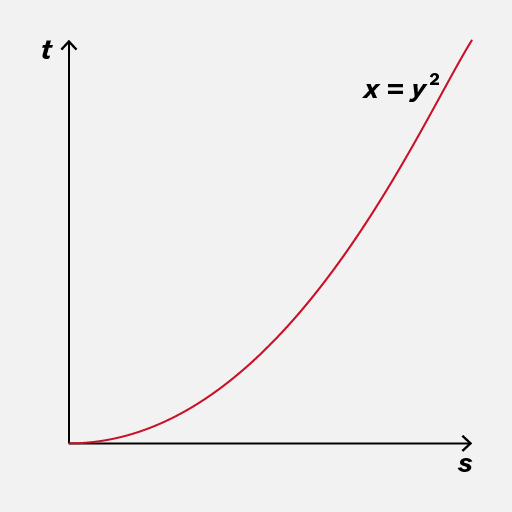
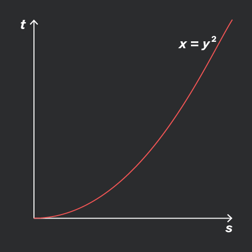
When writing down an equation of a line or curve, use the correct letters as they appear on the graph.
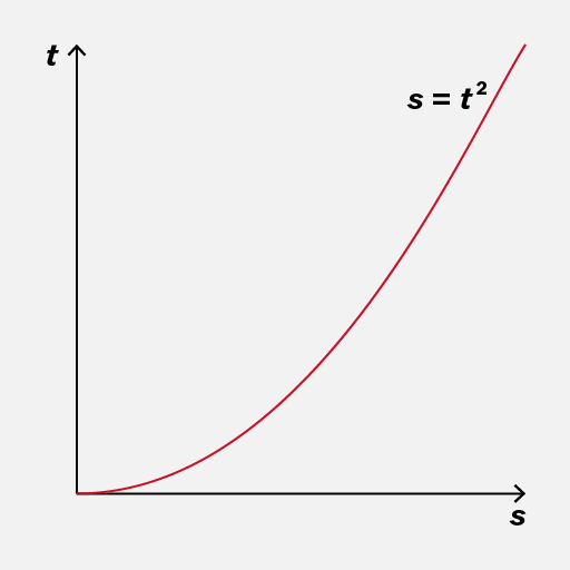
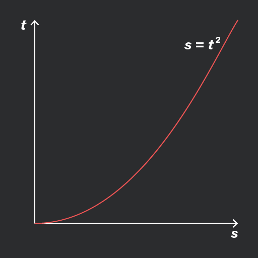
A graph depicting the relationship between time (t) and distance (s), with the curve representing the equation s = t². The vertical axis is labeled 't' and the horizontal axis is labeled 's'.
Do

Use the same letters for the variables as in the graph.

A graph showing a parabolic curve representing the equation x = y². The vertical axis is labeled 't' and the horizontal axis is labeled 's'. The curve rises steeply as it moves to the right.
Don't

Use and or different letters, if they were not used on the graph.

Add to favourites

A relationship between two quantities is proportional if one quantity is simply a multiple of the other. Any graph of this would show a straight line through the origin.

The equation of this graph would be , where is the gradient of the line and is also the constant of proportionality. For example, in the green and blue lines below the gradient is .
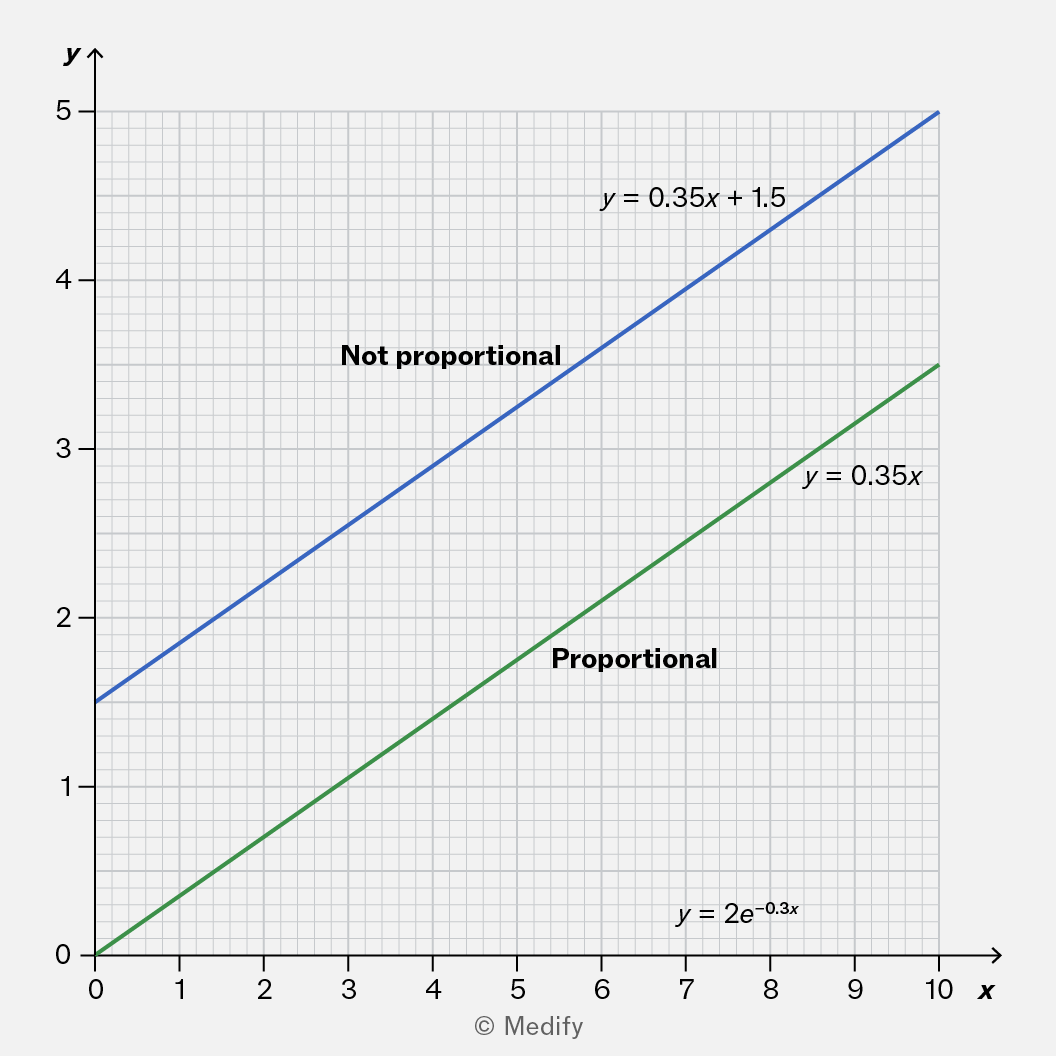
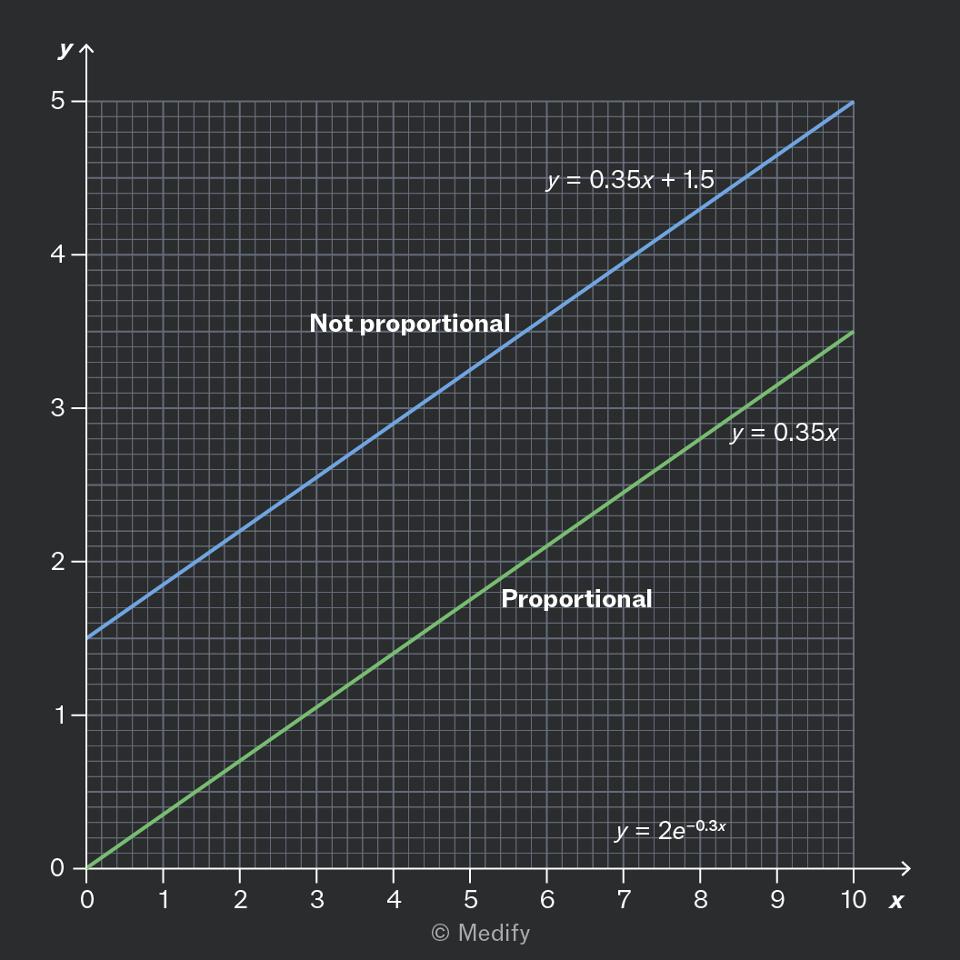
A graph displaying two lines: the blue line labeled 'Not proportional' represents the equation y = 0.35x + 1.5, while the green line labeled 'Proportional' represents the equation y = 0.35x. The graph has a grid background with x-axis ranging from 0 to 10 and y-axis from 0 to 5.

Graphs of the form are also straight lines. But unless the -intercept is zero, the line does not pass through the origin, and the graph does not show proportionality.

Add to favourites

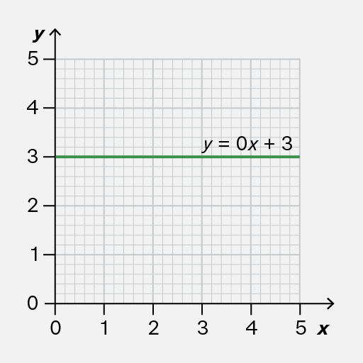
Most straight-line graphs should be written in the form where is the gradient.

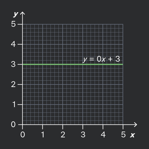
If the gradient is zero, it means that remains constant: it never changes.

In this case, which is better written as Keeping things simple with equations makes it easier to check your work and more quickly wrap your head around what comes next.
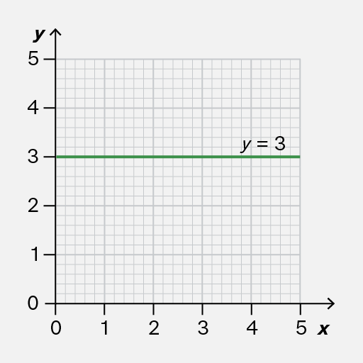
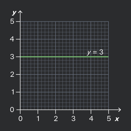
A Cartesian coordinate graph showing a horizontal line at y=3, spanning from x=0 to x=5, with grid lines in the background.
Do

Write the equation of a constant graph in the form

A Cartesian coordinate system with a horizontal line representing the equation y = 0x + 3, intersecting the y-axis at 3. The grid extends from 0 to 5 on the x-axis and 0 to 5 on the y-axis.
Don't

Include unnecessary terms such as in the equation of a constant graph.

Add to favourites

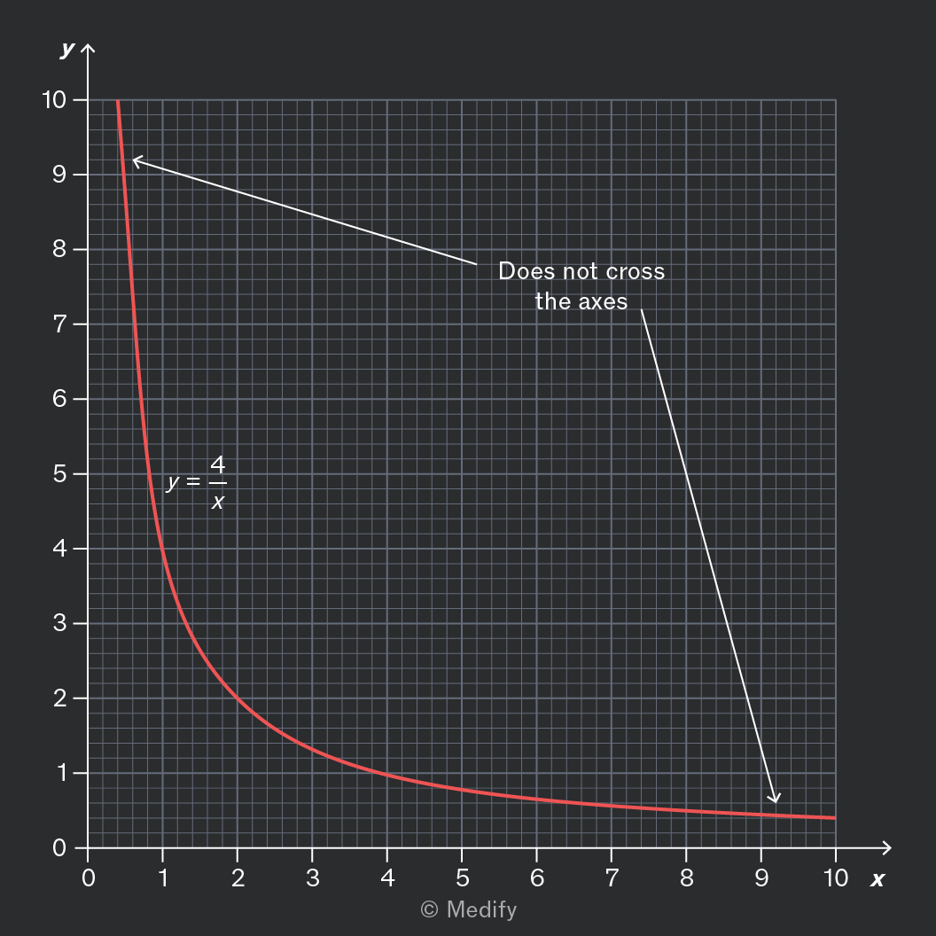
If and have a reciprocal relationship, it means that for some number . We can rearrange the equation:

Since division by zero is impossible, takes no value when , so the graph has no -intercept. In fact, the graph will not touch either axis.

If is large, then must be small, and vice versa, so the graph is very flat for large but very steep for close to zero.

You should be able to recognise reciprocal graphs by noticing these two properties.
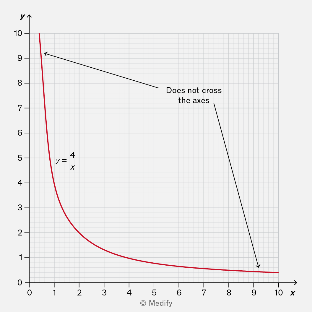
Graph of the function y = 4/x, showing a hyperbola that approaches the axes but never intersects them. The x-axis ranges from 0 to 10 and the y-axis ranges from 0 to 10, with annotations indicating that the curve does not cross the axes.
Add to favourites

You need to be able to recognise exponential graphs, which can show:

  • exponential growth, for example, a quantity that quadruples every hour
  • exponential decay, for example, a quantity that halves every second.

Examples of exponential graphs include:

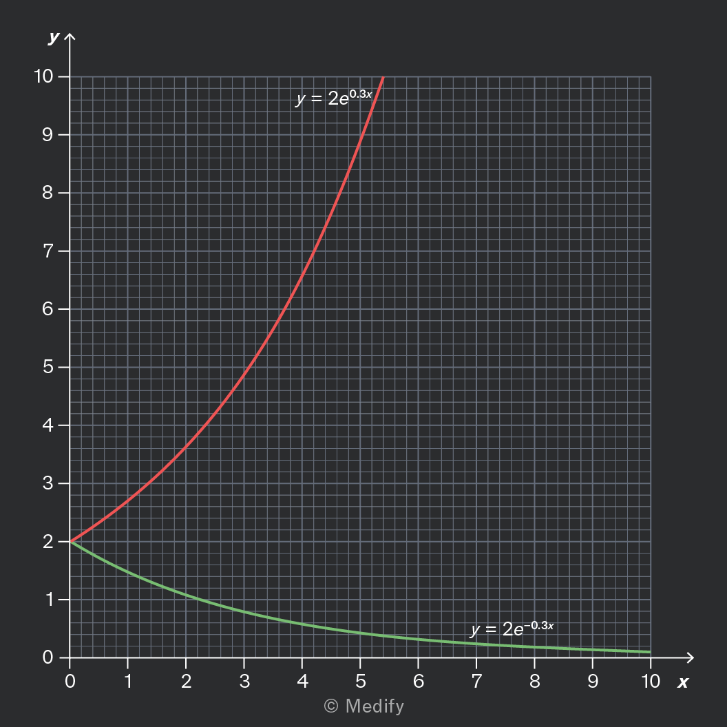
  • shows exponential growth, and the graph grows rapidly.
  • shows exponential decay, and the graph decreases towards zero without ever crossing the X axis.

In both cases, is the value of the x-intercept, because when ,
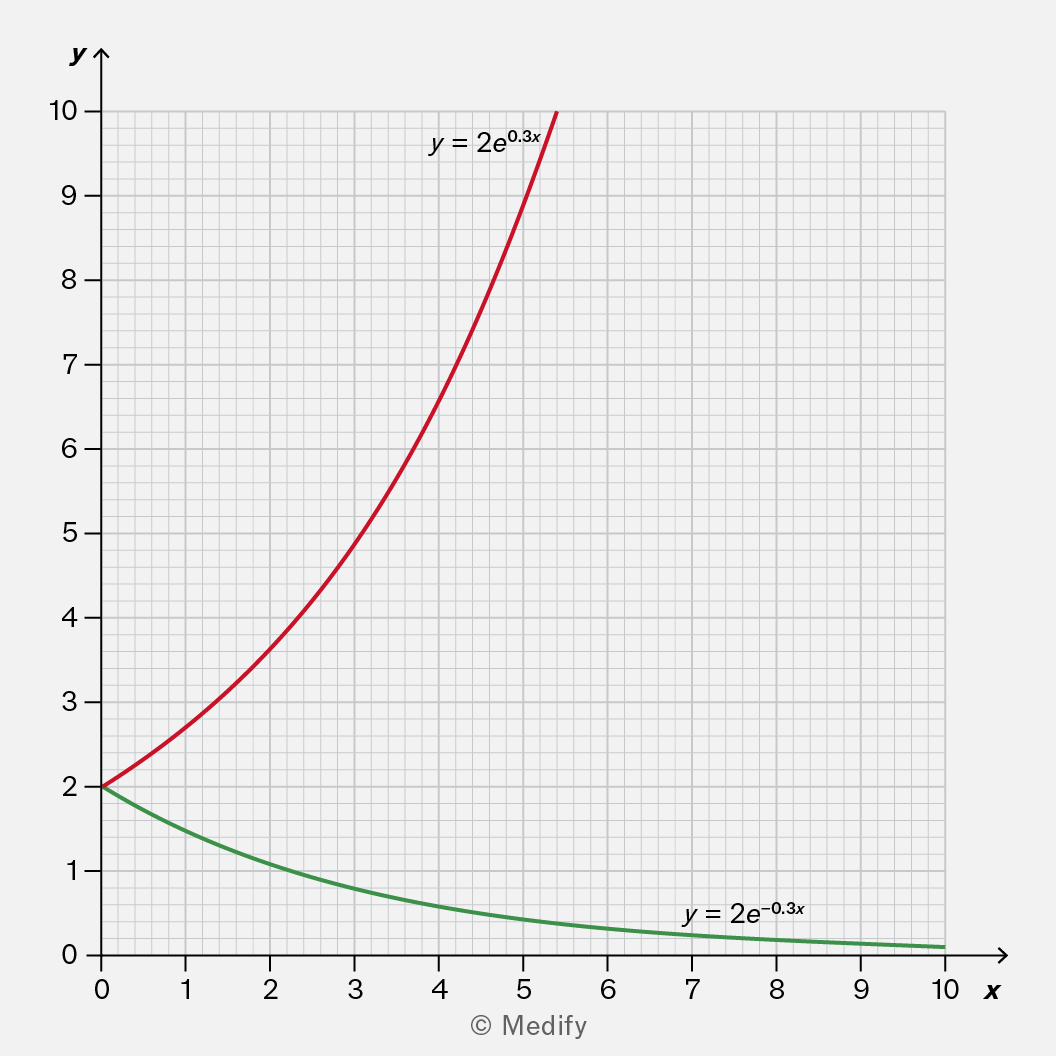
A graph showing two exponential functions. The red curve represents the equation y = 2e^(0.3x), which increases rapidly, while the green curve represents y = 2e^(-0.3x), which decreases towards zero. The x-axis ranges from 0 to 10 and the y-axis ranges from 0 to 10.

Here, the green graph decays towards zero, while the red graph grows exponentially.

Add to favourites

A quadratic graph has the shape of a parabola, resembling the letter U.

The equation of a quadratic graph is where and represent numbers that define the precise shape and position of the graph.

It is important to note:

  • is the value of the -intercept
  • If is made negative, the graph opens downwards; rather than a U-shape, it is upside-down like ∩.

It is useful to know:

  • if is large (positive or negative), then the parabola will be narrower
  • if is positive, the graph is sloping upwards at the -intercept. If is negative, the graph is sloping downwards at this point.
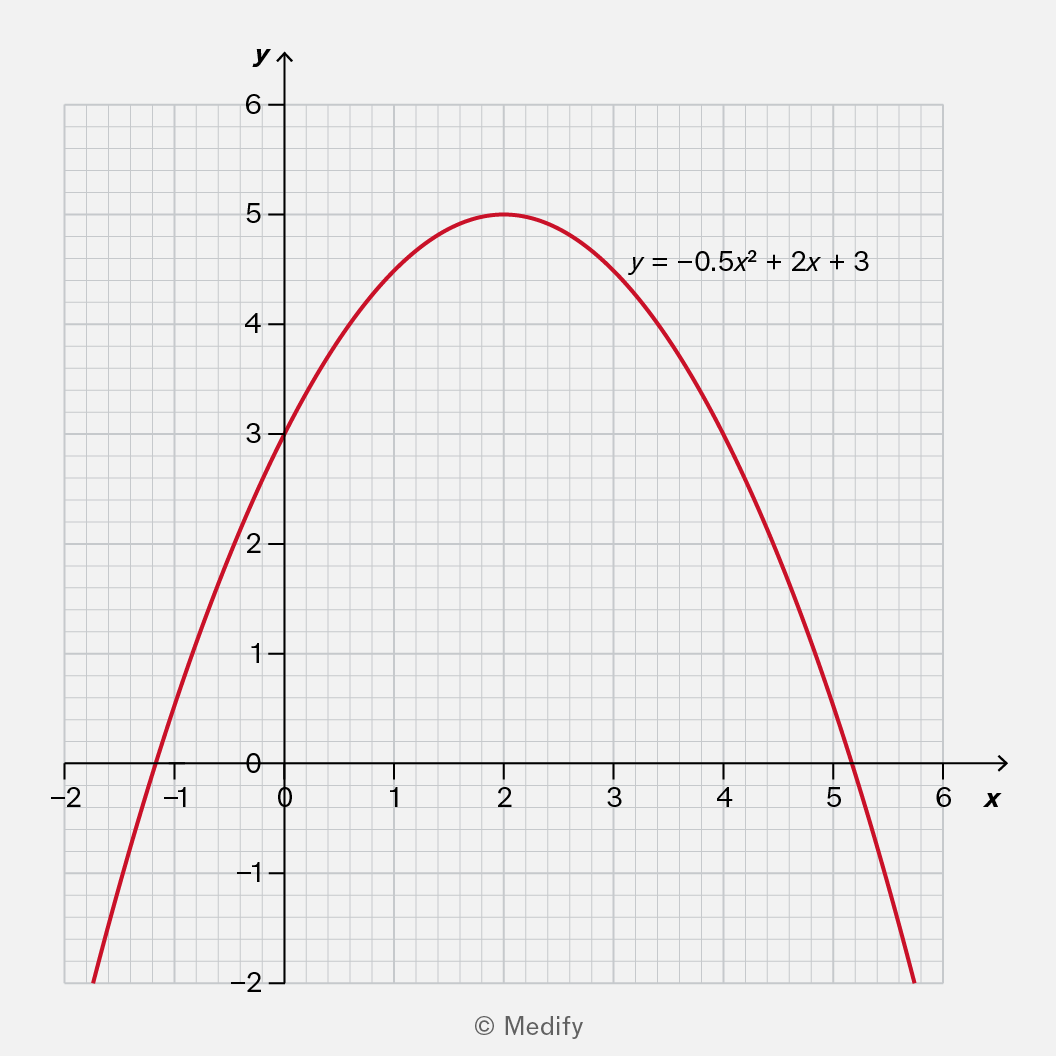
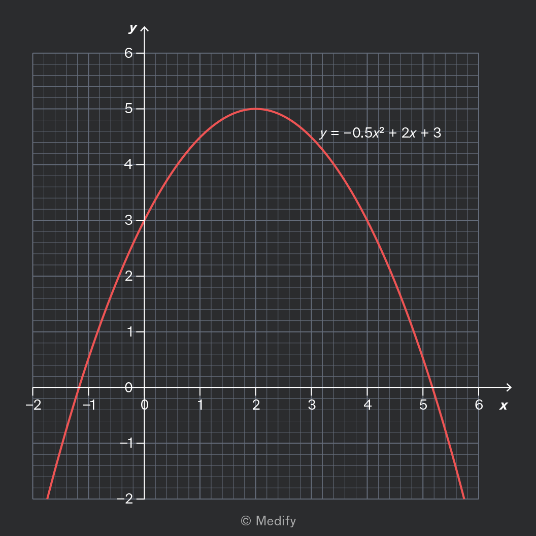
A graph of a quadratic function represented by the equation y = -0.5x² + 2x + 3. The curve opens downward, with the vertex at the highest point, and the axes are labeled with x and y values ranging from -2 to 6.
  • This parabola opens downwards, which tells you that the coefficient of is negative.
  • The graph is not very steep, which indicates that is not large. In fact,
  • The -intercept is which tells you that the constant term,
  • At the -intercept, the graph slopes upwards, so we know that In fact,
Add to favourites

A straight line through the origin tells you that is proportional to

Sometimes you will see a graph that starts at the origin and curves upwards. Graphs like this tell you that is proportional to a power of

This can be written as for some number It can also be written as where is some constant of proportionality.
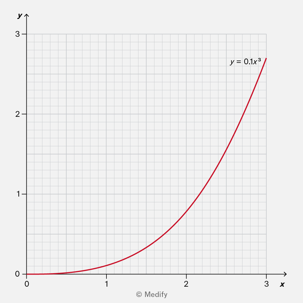
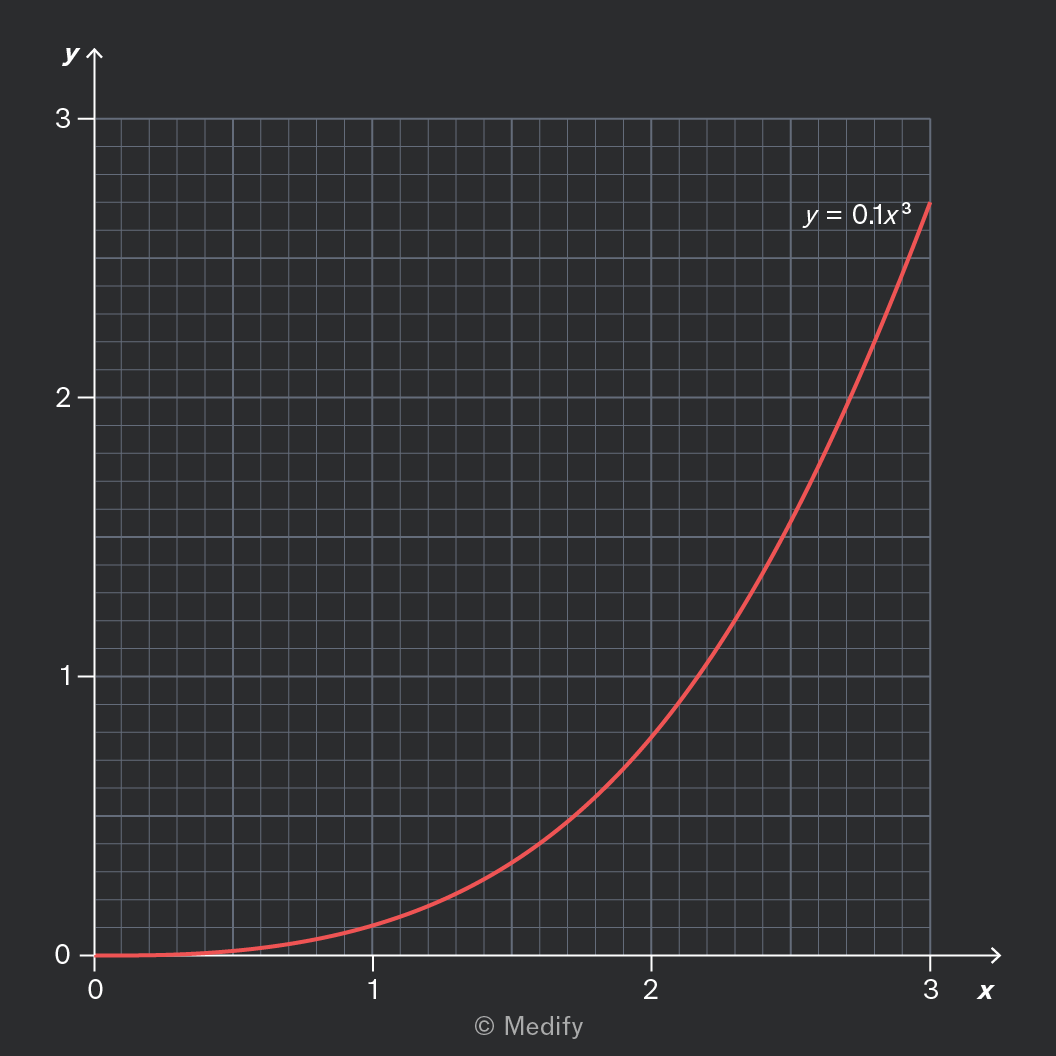
A graph depicting the cubic function y = 0.1x^3, with the x-axis ranging from 0 to 3 and the y-axis from 0 to 3. The curve starts near the origin and rises steeply, illustrating the growth of the function.

An example of a power relationship is shown in the graph above. The equation of the line is where is proportional to and the constant of proportionality is

It is challenging to determine these exact values solely by examining the graph. Luckily, you won’t need to do that!

Add to favourites

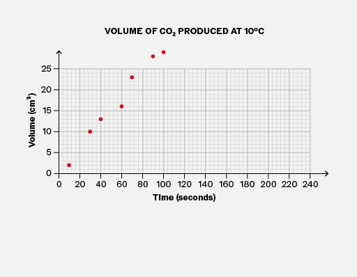
Graphs are for communicating information to other people, so clear labelling is crucial.

Always remember to include a brief title for the graph, and axis labels (including units) to clarify what measurements the data represents.
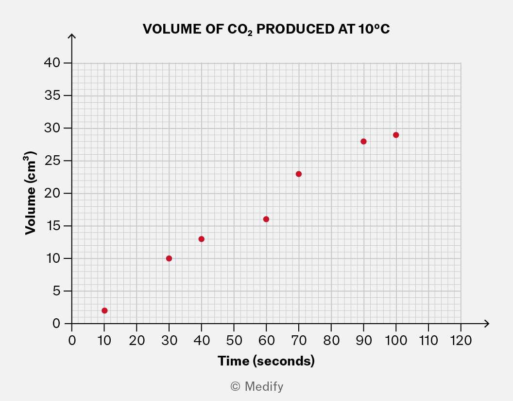
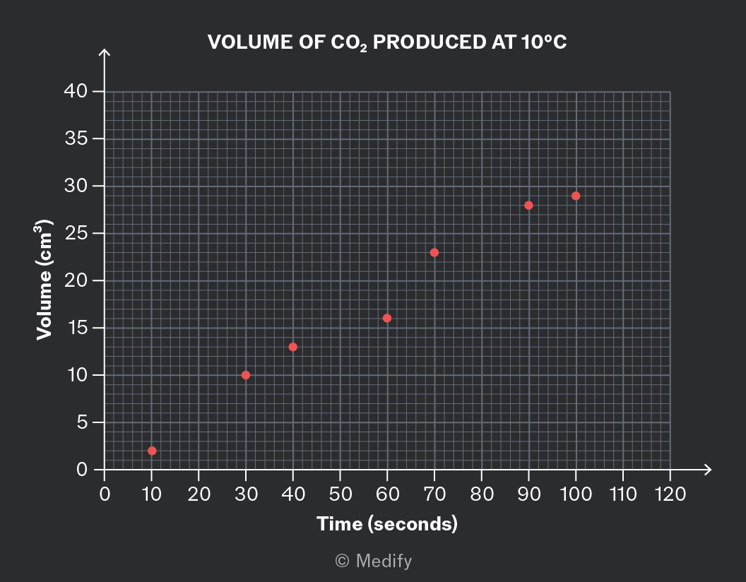
A graph titled 'VOLUME OF CO2 PRODUCED AT 10°C'. The x-axis is labeled 'Time (seconds)' with values from 0 to 120. The y-axis is labeled 'Volume (cm³)' with values from 0 to 40. There are seven red markers plotted: approximately (10, 5), (30, 10), (40, 15), (60, 20), (80, 25), (90, 30), and (100, 35).

This graph shows the approximate volume of gas produced two minutes after the experiment started.

This graph has a clear title and axis labels, which allow us to answer questions like this confidently.

It is important to note that you may lose marks in your exam if you draw a graph that omits these features.

Add to favourites

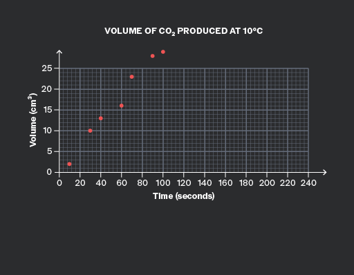
To make your graphs easy to read, it is important to choose suitable scales for both axes.
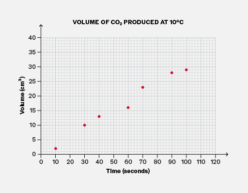
A graph titled 'VOLUME OF CO2 PRODUCED AT 10°C'. The x-axis is labeled 'Time (seconds)' with values ranging from 0 to 120 at intervals of 10. The y-axis is labeled 'Volume (cm³)' with values ranging from 0 to 40 at intervals of 5. Seven red markers are plotted: approximately (10, 3), (20, 7), (30, 10), (50, 15), (70, 20), (90, 27), and (110, 30).
Do

Choose suitable scales for the axes, so that the data fills most of the height and width of the graph area, and none of the data points are outside the area.

A graph titled 'VOLUME OF CO2 PRODUCED AT 10°C' shows the volume of CO2 in cm³ on the y-axis and time in seconds on the x-axis. The y-axis is labeled 'Volume (cm³)' with increments of 5 up to 25. The x-axis is labeled 'Time (seconds)' with increments of 20 up to 240. Seven red markers are plotted on the graph: approximately (0,0), (20,5), (40,10), (60,15), (80,18), (100,22), and (120,25), illustrating an increasing trend.
Don't

Choose scales for the axes that are too wide, like the horizontal axis here. It cramps the data and risks inaccuracy when reading values and drawing trendlines.

Choose scales too narrow so that data points fall outside the graph area, like the vertical axis here.

Add to favourites

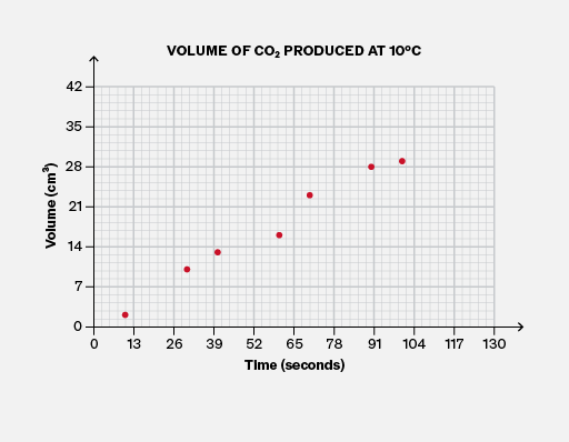
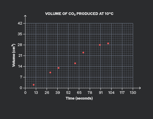
To make your graphs easy to read, it is important to choose suitable scales for both axes. It is usually best to use multiples of values related to British coins and notes, such as 1, 10, 100, …, 2, 20, 200, …, 5, 50, 500.
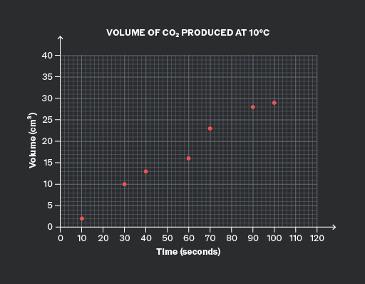
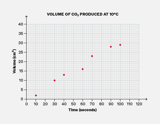
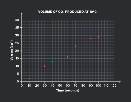
A graph titled 'VOLUME OF CO2 PRODUCED AT 10°C' with 'Volume (cm³)' on the y-axis and 'Time (seconds)' on the x-axis. The y-axis ranges from 0 to 40, and the x-axis ranges from 0 to 120. There are eight visible red markers plotted on the graph: approximately at (10, 3), (20, 7), (30, 9), (40, 14), (60, 18), (80, 25), (90, 28), and (110, 32). The plotted points show an upward trend over time.
Do

Choose a simple multiple to use on both axes.

Here, the horizontal scale uses multiples of 20, and the vertical axis uses multiples of 5.

A graph titled 'Volume of CO2 Produced at 10°C'. The x-axis is labeled 'Time (seconds)' with values from 0 to 130. The y-axis is labeled 'Volume (cm³)' with values from 0 to 42. There are seven plotted markers: approximately (13, 4), (26, 8), (39, 14), (52, 18), (65, 21), (78, 28), and (104, 32).
Don't

Choose inconvenient multiples for either axis.

Here, the horizontal axis uses multiples of 13, and the vertical axis uses multiples of 7.

Both axes are difficult to read. Try reading the middle data point! This could waste time and cause errors in an exam situation.

Add to favourites

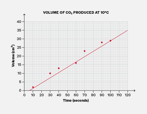
Lines of best fit (and curves) usually have a similar number of data points above the line (or curve) as below it. If you draw a line of best fit for which this is not true, you should reconsider whether it is accurate!

It is useful to know that in very few extreme cases, the number of data points above and below the line of best fit could be quite different. But this is rare!
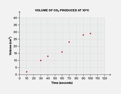
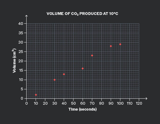
A scatter plot titled 'VOLUME OF CO2 PRODUCED AT 10°C'. The x-axis is labeled 'Time (seconds)' with values from 0 to 120 in intervals of 10. The y-axis is labeled 'Volume (cm³)' with values from 0 to 40 in intervals of 5. There are seven visible plotted markers representing data points: (10, 2), (20, 5), (30, 10), (50, 15), (70, 20), (90, 25), and (100, 30).
Do

Ensure there is a similar number of data points above and below the line of best fit.

Here, four points are above the line and three points are below it, which is quite balanced.

A graph titled 'VOLUME OF CO2 PRODUCED AT 10°C' with the x-axis labeled 'Time (seconds)' ranging from 0 to 120, and the y-axis labeled 'Volume (cm³)' ranging from 0 to 40. There are nine visible plotted markers at approximately (0, 0), (10, 5), (20, 10), (30, 15), (40, 20), (60, 25), (70, 30), (90, 35), and (100, 37). A red line connects these points, showing an upward trend.
Don't

Allow an imbalance between the amount of data above the line and below the line.

Here, only one of the seven points is below the line, so it is unlikely to be suitable for the line of best fit!

Add to favourites

You must draw lines of best fit accurately, as you may need to read precise values from them. Therefore, it is important to use a ruler or other straight edge.

Make sure you bring one to your exam!
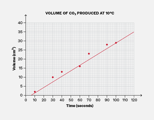
A graph titled 'VOLUME OF CO2 PRODUCED AT 10°C' with the x-axis labeled 'Time (seconds)' ranging from 0 to 120 and the y-axis labeled 'Volume (cm³)' ranging from 0 to 40. There are eight plotted red markers approximately at (0, 0), (10, 5), (20, 10), (30, 15), (40, 20), (60, 25), (80, 30), and (100, 35). A red line connects these markers, indicating a trend. The grid lines provide a reference for the plotted data.
Do

Use a ruler or straight edge when drawing a line of best fit.

A graph titled 'VOLUME OF CO2 PRODUCED AT 10°C' shows volume in cm³ on the y-axis and time in seconds on the x-axis. The y-axis ranges from 0 to 40 cm³, and the x-axis ranges from 0 to 120 seconds. Plotted red markers represent data points at approximately (10, 2), (20, 5), (30, 8), (40, 12), (50, 17), (60, 22), (80, 26), (90, 30), and (100, 33). A red line connects these markers, showing an increasing trend. The graph background has a grid pattern.
Don't

Attempt to draw a freehand line of best fit; it will probably not be accurate! You could lose easy marks for carelessness.

Add to favourites

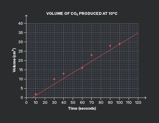
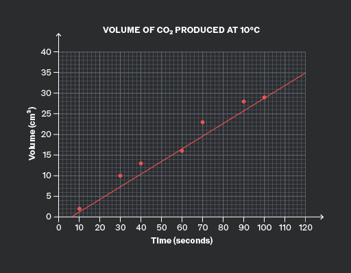
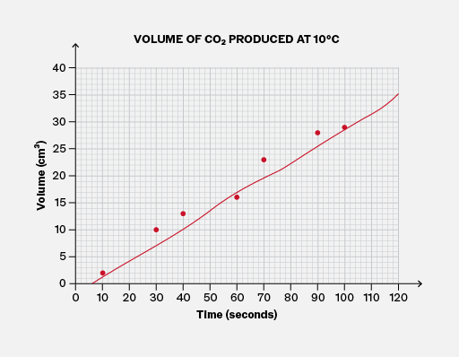
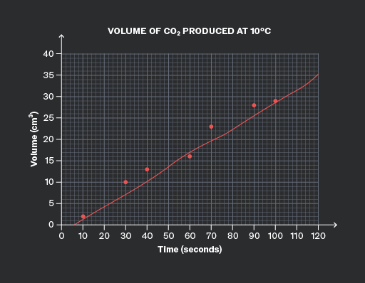
For data that follows a linear trend, you should draw a straight line of best fit through the data, using a ruler.

Never join the data dot-to-dot unless you are sure that the trend is not linear. For example, monthly climate data does not follow a linear trend.

Add to favourites

It is important to note that exam questions may ask you to interpolate, estimate, or predict values from a graph that shows a clear trend.

You should do this by drawing a line of best fit (or the curve) and reading values from that, rather than reading individual data points.

This is because the data points will fall above or below the line (or curve) due to unrelated factors (known as “noise”), such as human error. The line (or curve) reduces the effect of this noise.
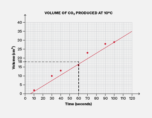
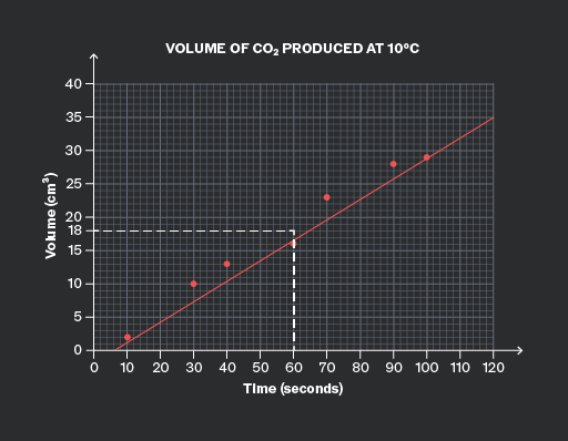
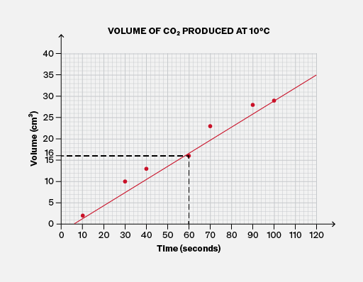
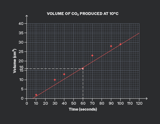
A graph titled 'VOLUME OF CO2 PRODUCED AT 10°C' with the x-axis labeled 'Time (seconds)' ranging from 0 to 120 and the y-axis labeled 'Volume (cm³)' ranging from 0 to 40. Six red data markers are plotted approximately at (0, 0), (20, 5), (40, 10), (60, 18), (80, 25), and (100, 30). A red line connects these points. There is a black dashed line forming a right triangle, highlighting the point at (60, 18).
Do

Use the line of best fit to directly estimate any values on the graph. This reduces the impact of noise in the data.

A graph titled 'VOLUME OF CO2 PRODUCED AT 10°C' with 'Time (seconds)' on the x-axis and 'Volume (cm³)' on the y-axis. The x-axis ranges from 0 to 120 seconds, and the y-axis ranges from 0 to 40 cm³. Plotted data points are shown as red dots at approximately (10, 5), (20, 10), (30, 15), (40, 17), (50, 22), (60, 25), (70, 30), (80, 32), (90, 35). A red line connects these points. A dashed black line extends horizontally from the y-axis at 20 cm³ to the red line and vertically down to the x-axis around 50 seconds.
Don't

Don’t ignore the line of best fit when the question asks you to interpolate, predict, or estimate values.

Add to favourites

Question walkthrough

Draw a line of best fit to extrapolate from data.

Draws a line of best fit through weight-extension data for an elastic fibre, then extends it to the y-axis to find its natural length when no weight is attached.

Question walkthrough

Draw a curve to extrapolate from data.

Draws a smooth curve of best fit through non-linear data, then uses it to extrapolate a prediction for lemonade sales at a forecast temperature.

In some scientific contexts, it is clear that any line of best fit (or curve) must pass through the origin. Some examples of where the graph must pass through the origin:

  • In Biology and Chemistry, in rate–concentration graphs, because when the concentration of the reactant is zero, the reaction does not happen.
  • In Physics, stress–strain graphs, because when no force is applied to the material, the material has zero deformation.
  • In any context, when a quantity has an initial value of zero.

You should use your scientific understanding to identify these cases and ensure that any line of best fit (or curve) passes through the origin.

It is important to note that in many other scenarios, there is no reason to expect that the line (or curve) would pass through the origin.
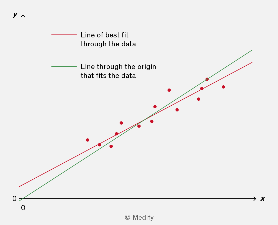
The image shows a graph with x-axis labeled 'x' and y-axis labeled 'y', both starting at 0. Red data points are scattered upwards on the graph. A red line labeled 'Line of best fit through the data' and a green line labeled 'Line through the origin that fits the data' are drawn through the data points. The red line is slightly lower than the green line. The green line passes through the origin (0,0), while the red line does not. The lines represent different methods of fitting the data points. The copyright is noted as © Medify.

For the data in this graph, which of the two lines should you use? It depends on the scientific context. You will need to choose!

Add to favourites

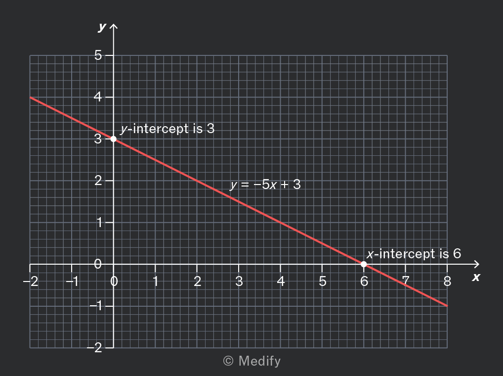
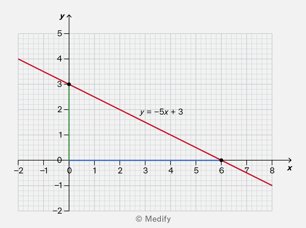
Where a straight-line graph crosses an axis, the crossing point is called an intercept.

The point where the graph crosses the vertical y-axis is called the y-intercept. This is often given the value when writing the equation of the straight line:

The point where the graph crosses the horizontal x-axis is called the x-intercept.
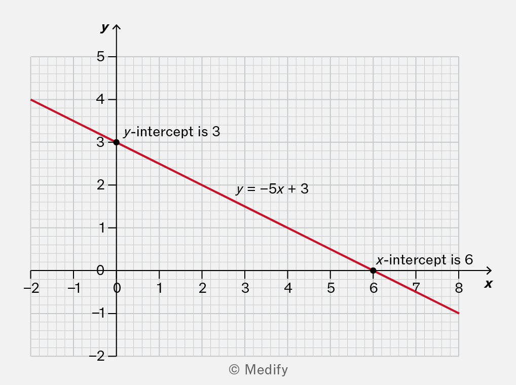
A graph showing a linear equation with a red line. The y-intercept is marked at 3, and the x-intercept is marked at 6. The equation of the line is y = -5x + 3.

Here, the y-intercept is 3, and the x-intercept is 6.

Add to favourites

To calculate the gradient of a graph, choose any two points and calculate:

If the two points are and the same expression can be written:

However, your answer may be inaccurate if you divide by a horizontal change that is too small. To avoid this, choose two points that are quite far apart.
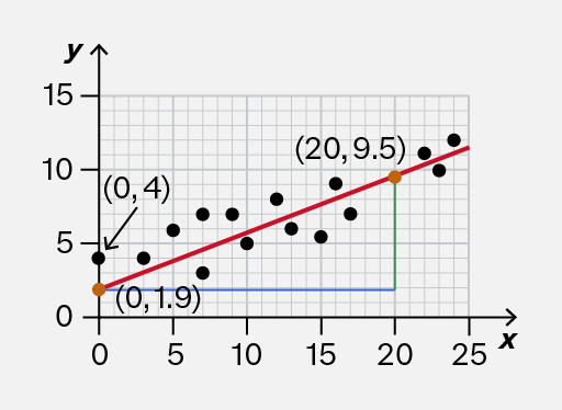
A graph with a red line representing a linear function, plotted on a grid. The x-axis ranges from 0 to 25 and the y-axis from 0 to 15. Two points are marked: one at (20, 9.5) with a green dot and another at (20, 1.9) with a green dot, connected by a vertical line. A blue horizontal line is drawn at y=20.
Do

Calculate the gradient using points that are far enough apart.

This is close to the true value of 0.383.

A graph with a red line representing a linear function plotted on a grid. The x-axis ranges from 0 to 25 and the y-axis ranges from 0 to 15. Two points are marked on the graph: one at (20, 9.5) and another at (20, 1.9), with green dots indicating their positions. A blue horizontal line is drawn at y = 20.
Don't

Calculate the gradient using points that are too close.

This is not accurate because the true value is 0.383.

Add to favourites

If a straight-line graph is sloping downwards, the gradient is negative.

You should use the same procedure to calculate the gradient, but make sure that the vertical change is negative because it’s a decrease.
A graph showing a linear equation y = -5x + 3. The y-axis is labeled with values from 0 to 5, and the x-axis is labeled with values from -2 to 8. The line intersects the y-axis at (0, 3) and the x-axis at (6, 0). The graph includes a grid for reference.

Add to favourites

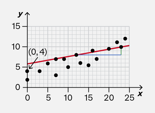
Sometimes you will be shown a graph of data from an experiment. The points follow a linear trend, and a (straight) line of best fit may be used to illustrate the trend.

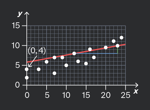
When estimating the slope and intercept of this graph, use the line itself, not the individual data points.
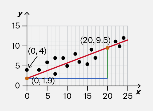
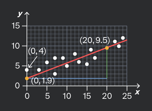
A scatter plot showing data points represented by black dots on a grid. A red line indicates the trend line, with coordinates labeled at two points: (0, 4) and (20, 9.5). A green vertical line and a blue horizontal line connect the point (20, 9.5) to the x-axis and y-axis, respectively. The origin (0, 0) is marked, along with the point (0, 1.9) on the y-axis.
Do

Use the line of best fit to calculate the slope (gradient) and intercept.

Here, the y-intercept is approximately 1.9, and the slope can be calculated accurately from points such as (0, 1.9) and (20, 9.5).

A scatter plot with a red trend line showing a positive correlation. The x-axis ranges from 0 to 25 and the y-axis from 0 to 15. Two specific points are labeled: (0, 4) with an arrow pointing to it, and (0, 1.9) marked with an orange dot. Another point (20, 9.5) is also indicated on the trend line.
Don't

Use individual data points to calculate the slope and intercept.

Here, the y-intercept is not 4; it’s approximately 1.9. The slope cannot be estimated accurately by using the two data points shown.

Add to favourites

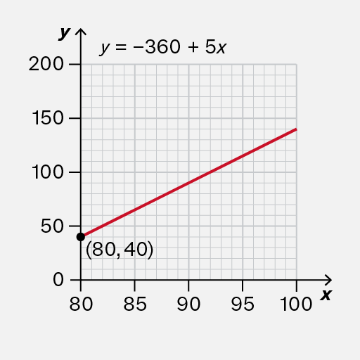
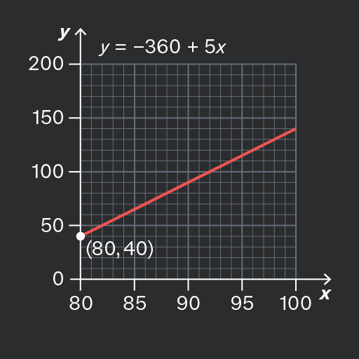
On most graphs, the horizontal axis starts at and therefore the y-intercept is on the vertical axis.

However, sometimes the horizontal axis is drawn differently. In these cases, you would need to do some further calculations to determine the y-intercept.
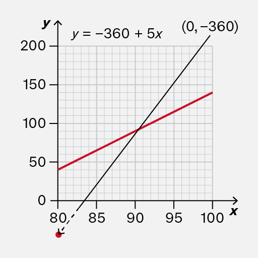
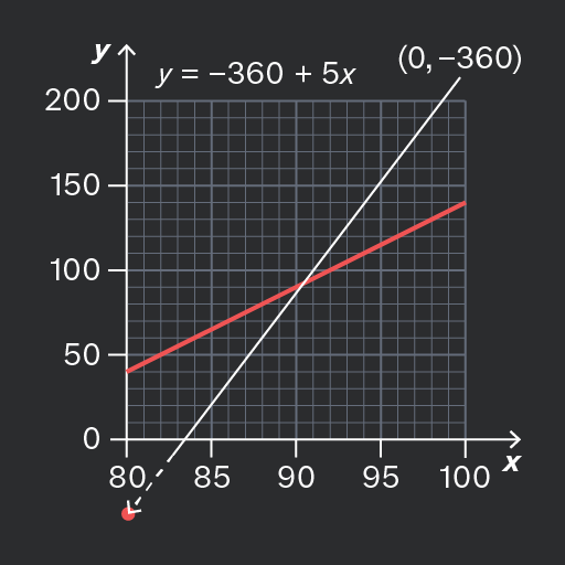
A graph showing a linear equation y = -360 + 5x. The x-axis ranges from 0 to 100 and the y-axis ranges from 0 to 200. A red line represents the equation, intersecting the y-axis at the point (0, -360). A point is marked on the x-axis at approximately 80.
Do

Notice that the y-intercept is not shown on this graph.

In fact, it is −360, which would require some effort to calculate.

A graph showing a linear equation y = -360 + 5x. The x-axis ranges from 80 to 100 and the y-axis ranges from 0 to 200. A red line represents the equation, with a point marked at (80, 40).
Don't

Attempt to read the y-intercept off the vertical axis, because on this particular graph, it is not aligned with

The y-intercept is not 40.

Add to favourites

Question walkthrough

Determine the slope and intercept of a linear graph

Using a drawn slope to determine a derived quantity from a linear graph.

Question walkthrough

Understand that y = mx + c represents a linear relationship

Translating an equation from numerical form to graphical form.

You may be asked to find the gradient of a straight-line graph, which is also known as the slope of the graph.

The gradient illustrates a rate of change, so some exam questions may use phrases similar to this instead. You need to recognise phrases about rates and interpret them as the gradient of a graph, if relevant.

You should also be aware that velocity (or speed) is the rate of change of position, and acceleration is the rate of change of velocity (or speed).

Add to favourites

If a straight-line graph has a positive gradient (it slopes upwards), then it shows a rate of increase.

If a straight-line graph has a negative gradient (it slopes downwards), then it shows a rate of decrease.

If the gradient of the straight line is zero (it is horizontal), then it shows that the quantity is not changing – it is constant.
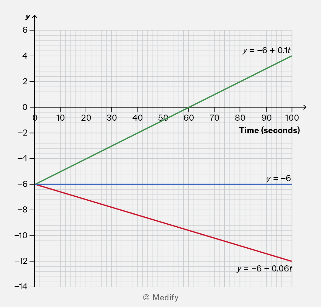
A graph showing three linear equations plotted against time in seconds on the x-axis and y-values on the y-axis. The green line represents the equation y = -6 + 0.1t, the blue line is y = -6, and the red line is y = -6 - 0.06t. The graph includes a grid for reference.

The green line has a gradient of 0.1. It shows an increase of 0.1 units per second.
The blue line has a gradient of zero. It shows that the quantity is constant.
The red line has a gradient of −0.06. It shows a decrease of 0.06 units per second.

Add to favourites

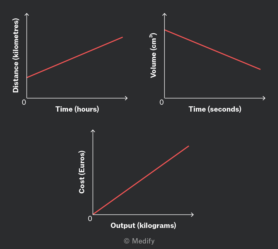
The units for a rate of change can be written in words by arranging the units from the axes:
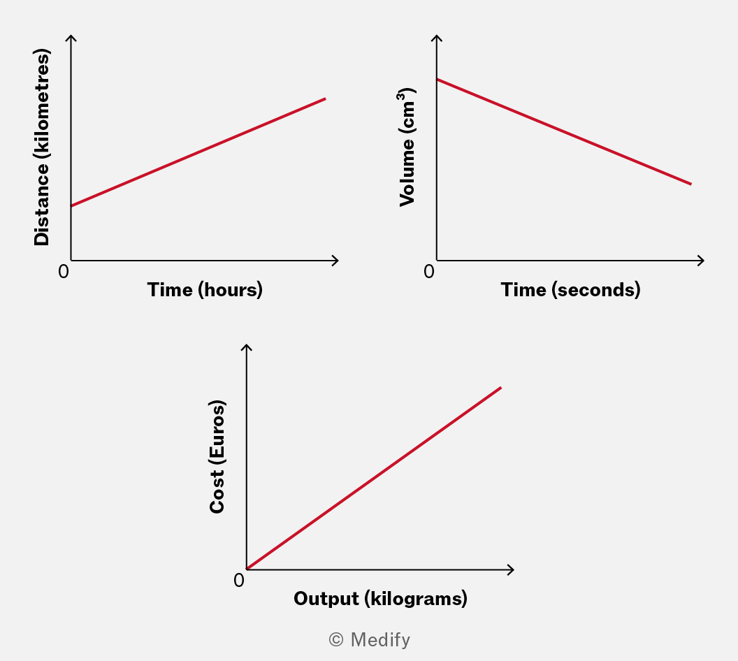
Three graphs illustrating different relationships: the first graph shows a linear increase in distance (kilometres) over time (hours), the second graph depicts a decrease in volume (cm³) over time (seconds), and the third graph represents a linear increase in cost (Euros) relative to output (kilograms).

Examples of this include:

  • kilometres per hour (or or )
  • cubic centimetres per second (or or )
  • Euros per kilogram (or € or €)

As noted in the examples, you may abbreviate these units in various ways to reduce the amount you need to write.

Exam boards generally accept both formats because they’re both scientifically correct ways to express the same thing. The key is being consistent and clear in your notation.

Add to favourites

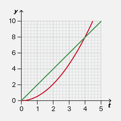
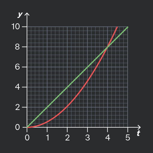
On a straight-line graph, the gradient is the same everywhere. The graph describes a quantity that always changes at the same rate.

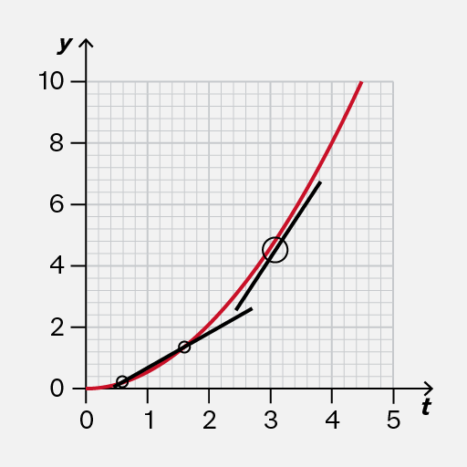
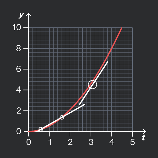
On a curve, the gradient is changing. The curve doesn’t rise or fall evenly; it changes based on the X-axis value.
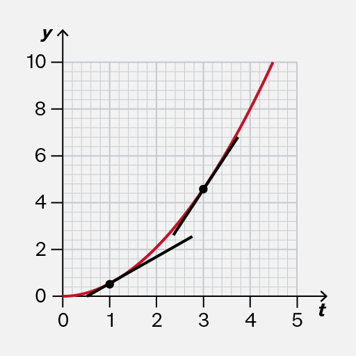
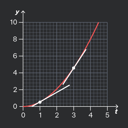
The graph displays a plot with a red curve and black line segments on a grid. The x-axis is labeled 't' with values from 0 to 5, and the y-axis is labeled 'y' with values from 0 to 10. Three black markers are visible on the black line segments at approximately (1, 1), (2, 3), and (3, 5). The red curve passes through the origin and continues upward beyond the plotted markers.
Do

Recognise that the gradient is changing.

The tangent lines in this example illustrate that the rate of change is greater when than when

The image shows a graph with an x-axis labeled 't' and a y-axis labeled 'y'. The x-axis ranges from 0 to 5, and the y-axis ranges from 0 to 10. There are two lines plotted on the graph. The red line starts at the origin (0,0) and curves upward, passing through approximately (1,1), (2,4), and (4,9). The green line starts at the origin (0,0) and follows a straight diagonal path, intersecting the y-axis at 10 and the x-axis at 5. The grid in the background aids in estimating the positions of the lines.
Don't

As the gradient is changing, do not use the straight line between any two points (such as and as shown on the image) to represent the rate of change at any moment.

Add to favourites

Question walkthrough

Draw and use the slope of a tangent to a curve as a measure of rate of change

Uses a tangent to a curve to estimate the instantaneous speed of a machinery component at a given time, by drawing the tangent and measuring its gradient between two points.

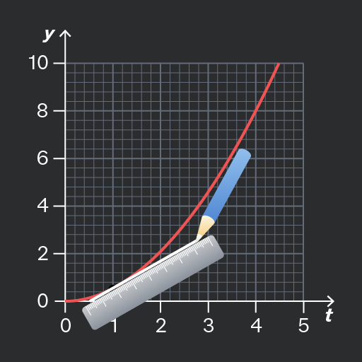
It can be difficult to draw the tangent line accurately! It should touch the curve without crossing it.

You should use a pencil so that you can easily erase a line if necessary.
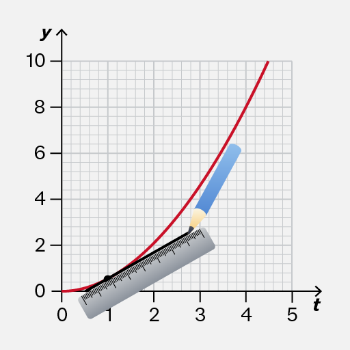
A graph with a grid background showing an upward curving red line. The x-axis is labeled 't' and ranges from 0 to 5. The y-axis is labeled 'y' and ranges from 0 to 10. A ruler and pencil are overlayed on the graph, aligned with the red curve between t = 1 and t = 3. The red line starts near the origin and curves upward as t increases, approximately passing through (1, 1), (2, 3), and (3, 5) based on the grid. No markers are present, and no numeric annotations are directly on the line.
Do

Carefully position your ruler about away from the curve to account for the width of your pencil.

A graph with a grid background showing two axes. The x-axis is labeled 't' and ranges from 0 to 5, while the y-axis is labeled 'y' and ranges from 0 to 10. The graph includes a red curve and a black line with three visible plotted markers. The markers are open circles located approximately at (1, 1), (2, 2), and (3, 3). The red curve starts near the origin and rises steeply, passing through the markers. A larger open circle is drawn around the marker at (3, 3).
Don't

The tangent should not cross the curve, nor leave a gap. Otherwise, it would be difficult to check whether your line has the same gradient as the curve.

Add to favourites

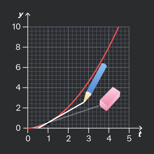
Sometimes, your first attempt at drawing a tangent line may not be accurate. For example, the tangent line could cross the curve.

If that happens, you should erase the inaccurate tangent line and try again.

You should use a pencil so that it is convenient to erase a line if necessary.
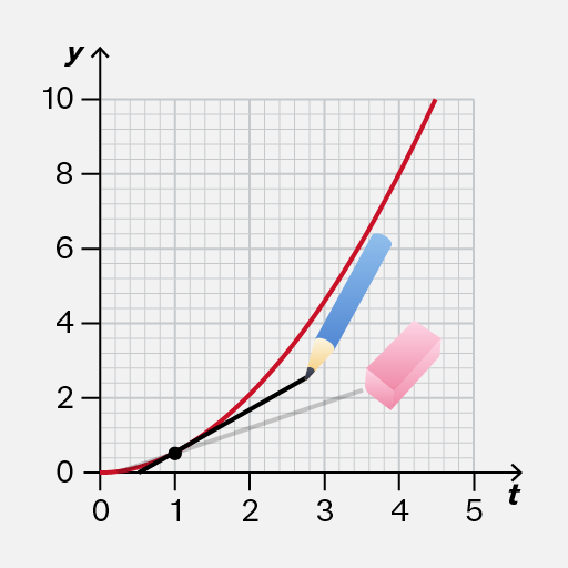
A graph with a y-axis labeled 'y' ranging from 0 to 10 and a t-axis labeled 't' ranging from 0 to 5. A red curve extends from the bottom left near the origin upward to the top right. A visible plotted marker is at approximately (1, 1) on the graph. A red line connects this point to the curve at approximately (3, 3). A blue pencil and a pink eraser are illustrated on the graph, overlapping the red line, suggesting a drawing or editing action. Gridlines are visible in the background.
Do

Use a pencil so that it is convenient to erase a line if you have not drawn it accurately.

Then you can try again to draw a better tangent line.

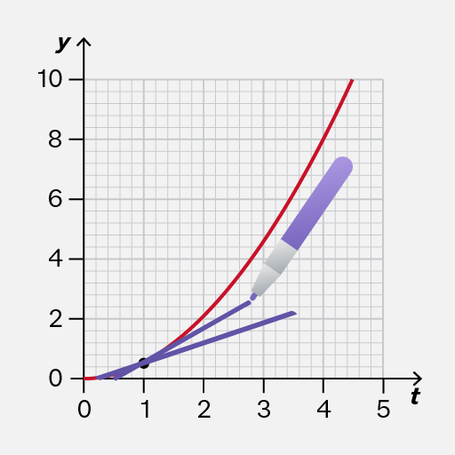
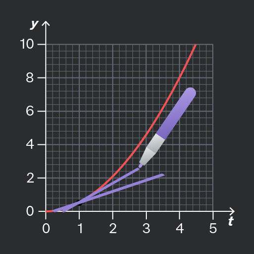
The image shows a graph with a grid background. The x-axis is labeled 't' and the y-axis is labeled 'y'. The x-axis ranges from 0 to 5, and the y-axis ranges from 0 to 10. A red curved line is plotted, increasing from approximately (0.5, 0) to (4.5, 8.5). A black dot is marked at approximately (1, 1.2) on the red line. A purple line extends from approximately (0.5, 0.5) to (3.5, 2.5) with a purple pen illustration pointing to it, near (3, 2).
Don't

Don’t use a thick pen because if your original attempt at a tangent line is inaccurate, you might not be able to see the original graph clearly to redraw an accurate line!

Add to favourites

You may be asked to find the instantaneous rate of change at a particular moment, or the average rate of change over a particular time interval.

It is important that you calculate the correct rate!
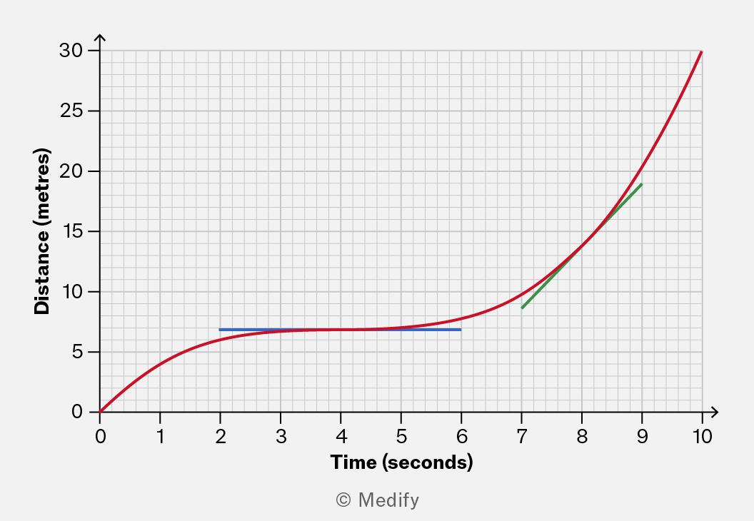
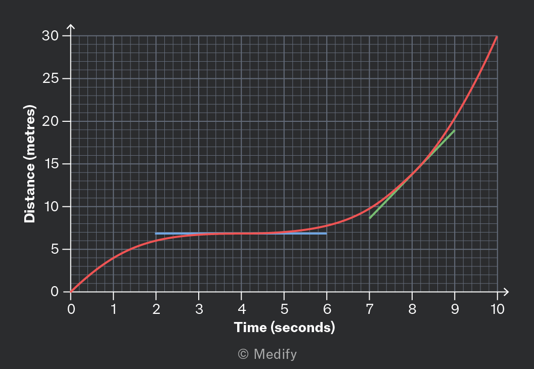
A graph showing the relationship between time (in seconds) and distance (in meters). The x-axis represents time from 0 to 10 seconds, while the y-axis represents distance from 0 to 30 meters. The curve indicates a gradual increase in distance over time, with sections highlighted in blue and green to denote specific intervals.

The example graph above shows a vehicle that travelled 30 metres in 10 seconds. Its average velocity was therefore over this interval.

However, at four seconds, the graph is horizontal, showing that the vehicle was not moving. At this moment, its instantaneous velocity was

Moreover, at eight seconds, the instantaneous velocity was about as illustrated by the green tangent line.

Add to favourites

Question walkthrough

Calculate an average rate of change

Determining the average rate of change of height from a graph.

Speed and velocity each describe the rate of change of position.

However, there is one important difference:

  • Speed is a scalar quantity; it is not affected by the direction of motion.
  • Velocity is a vector quantity. It is positive in the forward direction and negative in the backwards direction.

When considering velocity, consider whether the motion is forward or backwards.
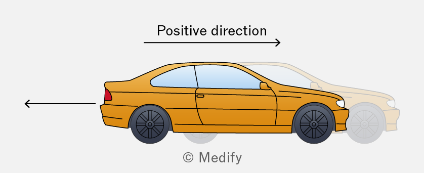
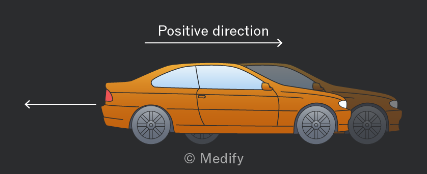
Illustration of a side view of an orange car with arrows indicating the positive direction of movement.

An example of this, is if we regard movement towards the right to be positive, when the car is moving in the opposite direction:

  • its speed is positive, (e.g. )
  • its velocity is negative, (e.g. )
Add to favourites

Recall:

  • Velocity is the rate of change of displacement (rate of change of position).
  • Acceleration is the rate of change of velocity.

These are vector quantities, so they can be positive or negative depending on the motion.

Add to favourites

The area under a graph sometimes has significance, although not always! You should be aware of the following examples:
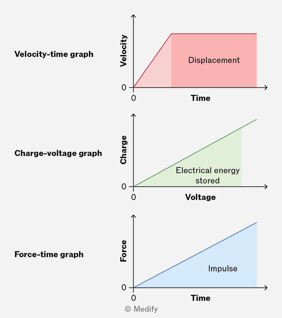
The image shows three separate graphs, each labeled and with axes described as follows: 1. Velocity-time graph: The x-axis is labeled 'Time' and the y-axis 'Velocity'. The graph shows a red line forming a right-angled trapezoid, with a shaded area labeled 'Displacement'. Both axes start at 0. 2. Charge-voltage graph: The x-axis is labeled 'Voltage' and the y-axis 'Charge'. The graph displays a green line forming a right-angled triangle, with a shaded area labeled 'Electrical energy stored'. Both axes start at 0. 3. Force-time graph: The x-axis is labeled 'Time' and the y-axis 'Force'. The graph features a blue line forming a right-angled triangle, with a shaded area labeled 'Impulse'. Both axes start at 0.
Add to favourites

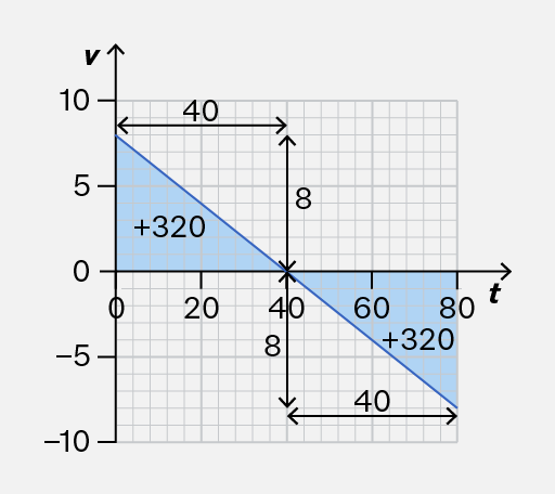
When calculating a quantity using the area under a graph, any areas beneath the horizontal axis count as negative. You should find the areas above the axis and subtract any areas beneath it.

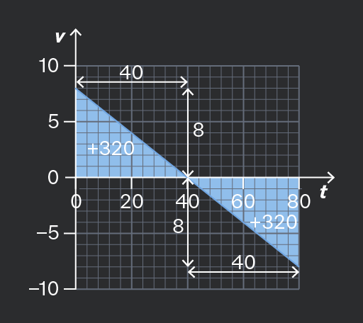
Consider the following velocity–time graph. How would you calculate the total displacement after seconds?
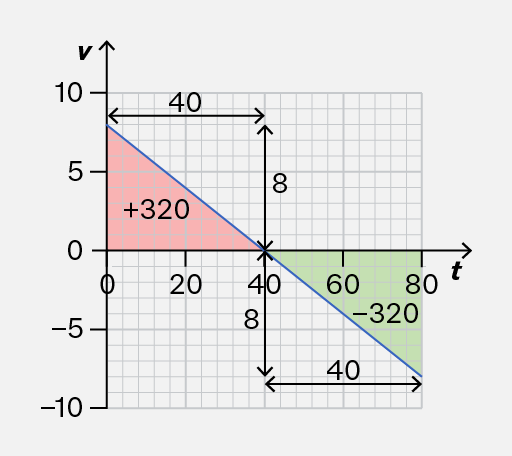
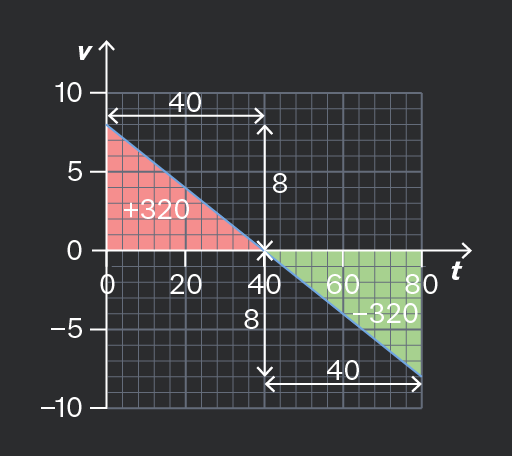
The image shows a graph with a grid background. The x-axis is labeled 't' and the y-axis is labeled 'v'. The y-axis ranges from -10 to 10 and the x-axis ranges from 0 to 80. A diagonal blue line runs from the top left to the bottom right of the graph, dividing it into two colored triangles. The left triangle is red with the annotation '+320' inside, and the right triangle is green with the annotation '-320'. The graph includes several black double-headed arrows with labels: '40' along the x-axis between 0 and 40, '40' along the x-axis between 40 and 80, '8' along the y-axis between 0 and 8, and '8' along the y-axis between -8 and 0. Another arrow labeled '8' is drawn vertically from 0 to 8 on the left side, and an arrow labeled '40' is drawn horizontally from 0 to 40 on the top. The grid lines are evenly spaced, and the graph is divided into smaller squares.
Do

Subtract areas that are below the axis.

Here, the displacement is: After seconds, the object is in the same horizontal position as it started.

The image is a graph with a grid background, featuring a diagonal blue line. The vertical axis is labeled 'v' with values marked at -10, -5, 0, 5, and 10. The horizontal axis is labeled 't' with values marked at 0, 20, 40, 60, and 80. The line slopes downward from left to right, intersecting the vertical axis at approximately 8 and the horizontal axis at approximately 40. There are two blue shaded triangles on the graph. The triangle on the left has a base along the vertical axis from 0 to 8 and a height of 40 along the horizontal axis. The triangle on the right has a base from 40 to 80 along the horizontal axis and a height of 8. Text annotations include '+320' within each triangle, '40' and '8' along the axes, and arrows indicating segment lengths and directions.
Don't

Add areas under the graph because they should count as negative.

Here, you should not add because the velocity after seconds was negative.

Add to favourites

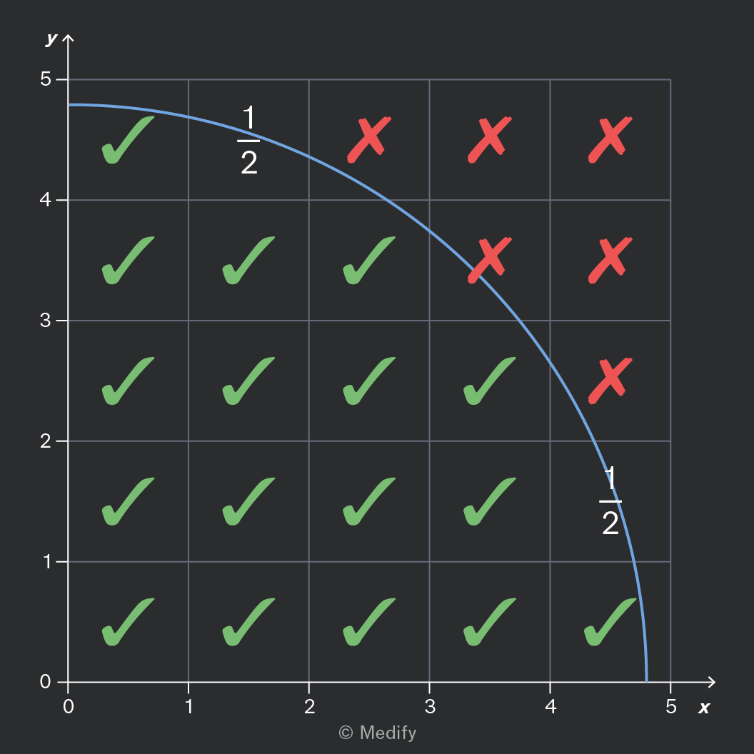
When finding the area under a graph by counting rectangles, your answer will be an estimate.

To get a good estimate, use the following rule:

  • If more than half of the rectangle is under the curve, include it.
  • If less than half of the rectangle is under the curve, don’t include it.
  • If you are not sure, because it is approximately half under the curve, count it as one-half.
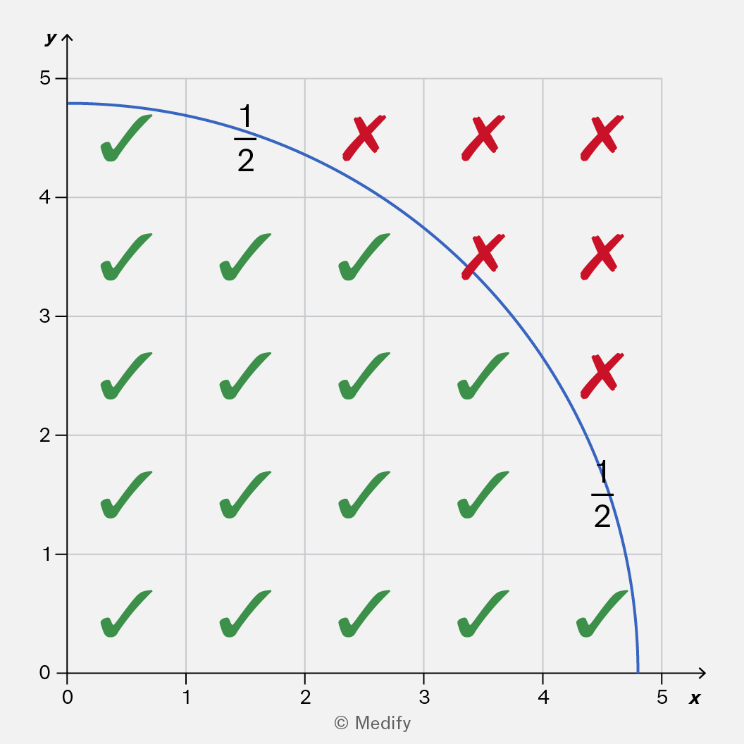
A graph with x-axis labeled 'x' ranging from 0 to 5 and y-axis labeled 'y' ranging from 0 to 5. A blue curve starts at approximately (0, 5) and ends at approximately (5, 0). The curve passes through (1, 4.5) and (4.5, 1). The grid is filled with checkmarks and crosses: Row 5: checkmark at 0 and 1, cross at 2, 3, 4, and 5. Row 4: checkmarks at 0, 1, 2, and 3, cross at 4 and 5. Row 3: checkmarks at 0, 1, 2, 3, and 4, cross at 5. Row 2: checkmarks at 0, 1, 2, 3, 4, and 5. Row 1: checkmarks at 0, 1, 2, 3, and 4, cross at 5. Annotations '1/2' appear near the curve at approximately (1, 4.5) and (4.5, 1).

You can approximate the area under this curve by counting the squares:

Add to favourites

Question walkthrough

Use geometry to find the area under a graph.

Uses the area under a velocity-time graph, split into a trapezium and a triangle, to find the distance of a town from the start of a train's journey, then interprets a negative area from a change in direction.

Question walkthrough

Count rectangles to estimate the area under a graph.

Uses the area under a charge-voltage graph to estimate the total energy discharged by a smartphone battery, by counting grid rectangles and multiplying by the energy each one represents.

The area under a graph can be calculated using graphical methods, like counting squares.

It is useful to note that the area can also be determined using calculus, although you won’t need to do this in your Science exams.

If you are studying A-level Mathematics, you may have seen that differentiation is a technique for finding the gradient function of a graph. The opposite is antidifferentiation or integration.
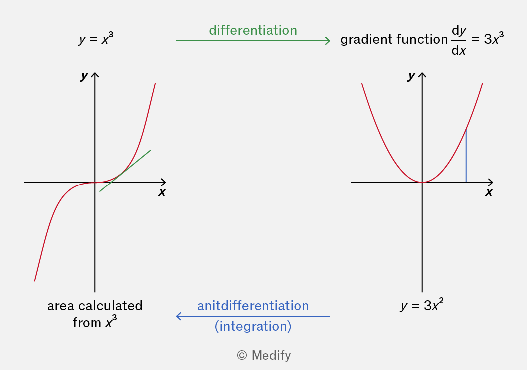
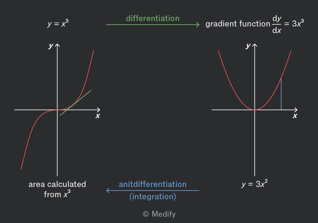
The image shows two graphs with their respective mathematical processes. On the left, the graph of y = x^3 is displayed, with a red curve intersecting the origin and extending in both positive and negative x directions. The x and y axes are labeled with 'x' and 'y'. A green tangent line indicates differentiation, labeled 'differentiation' pointing right to the right graph. Below the graph is the annotation 'area calculated from x^3'. On the right, the graph of y = 3x^2 is shown, with a red parabola opening upwards. The x and y axes are labeled 'x' and 'y'. Above the graph is the text 'gradient function dy/dx = 3x^3'. An arrow labeled 'antidifferentiation (integration)' points left back to the left graph.

The Fundamental Theorem of Calculus states that antidifferentiation of a function is the same as finding the area under the graph of that function.

In the image, the area under could be calculated either:

  • by graphical methods; or
  • by calculating the antiderivative and substituting in values for
Add to favourites

Some quantities (such as the number of radioactive particles in a large sample) decrease by the same proportion in each time interval. For example, the quantity might decrease by 20% each second, so that 80% remains.

The rate of decrease does not depend on previous values, only on its current value. Thus, it is sometimes described as memoryless.
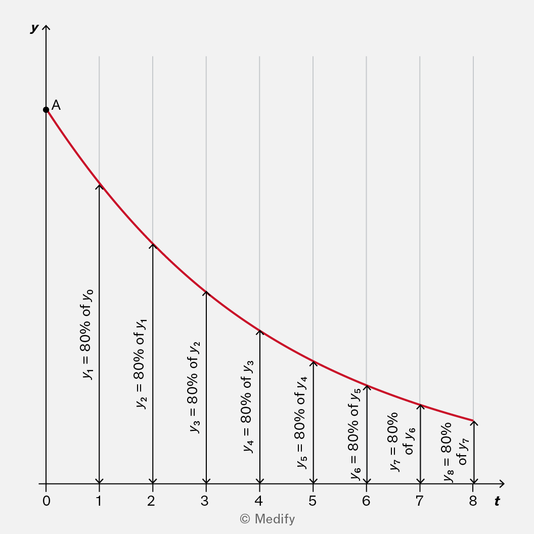
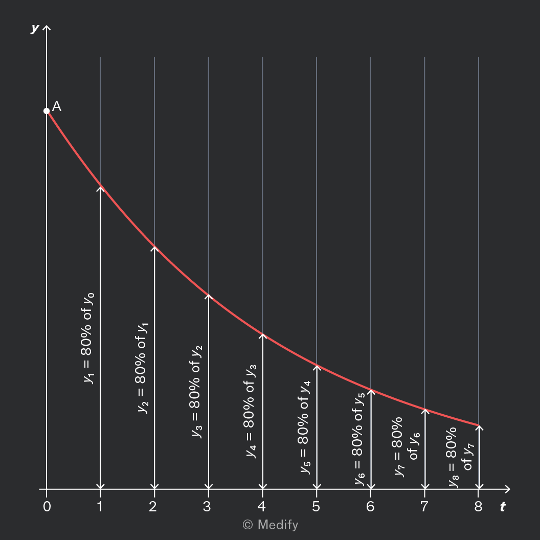
A graph with a downward curving red line, plotted on axes labeled 'y' (vertical) and 't' (horizontal). The horizontal axis 't' has tick marks at 0, 1, 2, 3, 4, 5, 6, 7, and 8. The vertical axis 'y' has a point labeled 'A' at the top. Along the curve, arrows and annotations indicate decreasing values: y1 = 80% of y0 at t=1, y2 = 80% of y1 at t=2, y3 = 80% of y2 at t=3, y4 = 80% of y3 at t=4, y5 = 80% of y4 at t=5, y6 = 80% of y5 at t=6, y7 = 80% of y6 at t=7, and y8 = 80% of y7 at t=8. The annotations are positioned along vertical arrows pointing downwards from each tick mark on the horizontal axis to the curve.

Memoryless decay is modelled using an exponential curve, as shown.

It always has the equation:

Where:

  • is the initial value (as shown), and
  • is the decay constant.

The greater the decay constant, the more rapid the decay.

Add to favourites

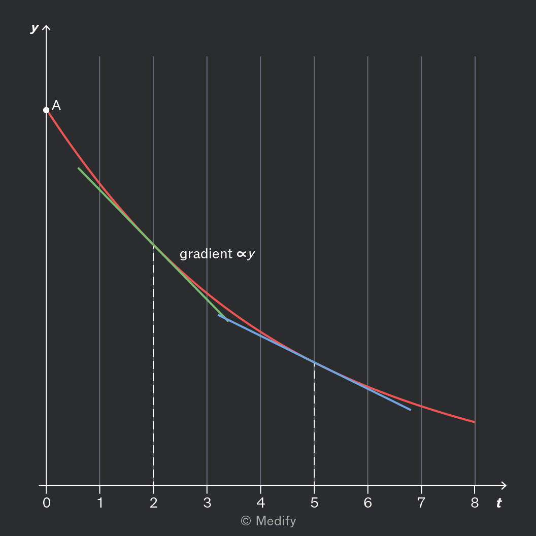
Some quantities (such as radioactive activity) decrease by the same proportion in each time interval.

This can be modelled by the differential equation:

Where:

  • is the decay constant, which depends on the rate of decay.

In formal notation, this can be written:

This always has the solution:

Where is the initial value.
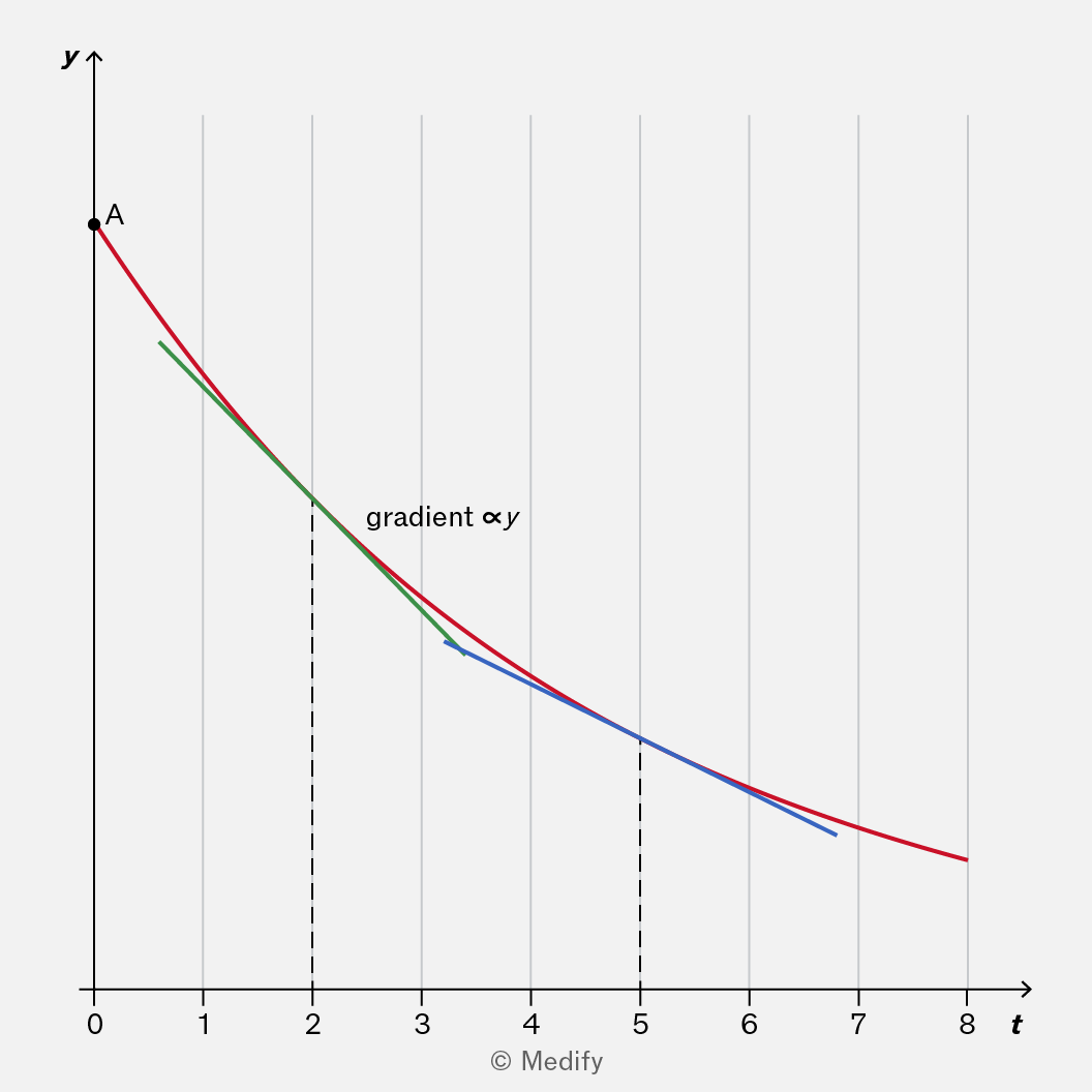
The image is a graph with the x-axis labeled 't' ranging from 0 to 8 and the y-axis labeled 'y'. There is a curved line plotted from the top left to bottom right, starting at point 'A' on the y-axis. The curve consists of three segments: red, green, and blue. The red segment starts at 'A', followed by a green segment, and then a blue segment. There is an annotation 'gradient ∝ y' near the green segment. Vertical dashed lines are present at approximately t=2 and t=5. The graph is marked with '© Medify' at the bottom.

Observe in the graph above that the gradient is always proportional to the value of as expected!

Add to favourites

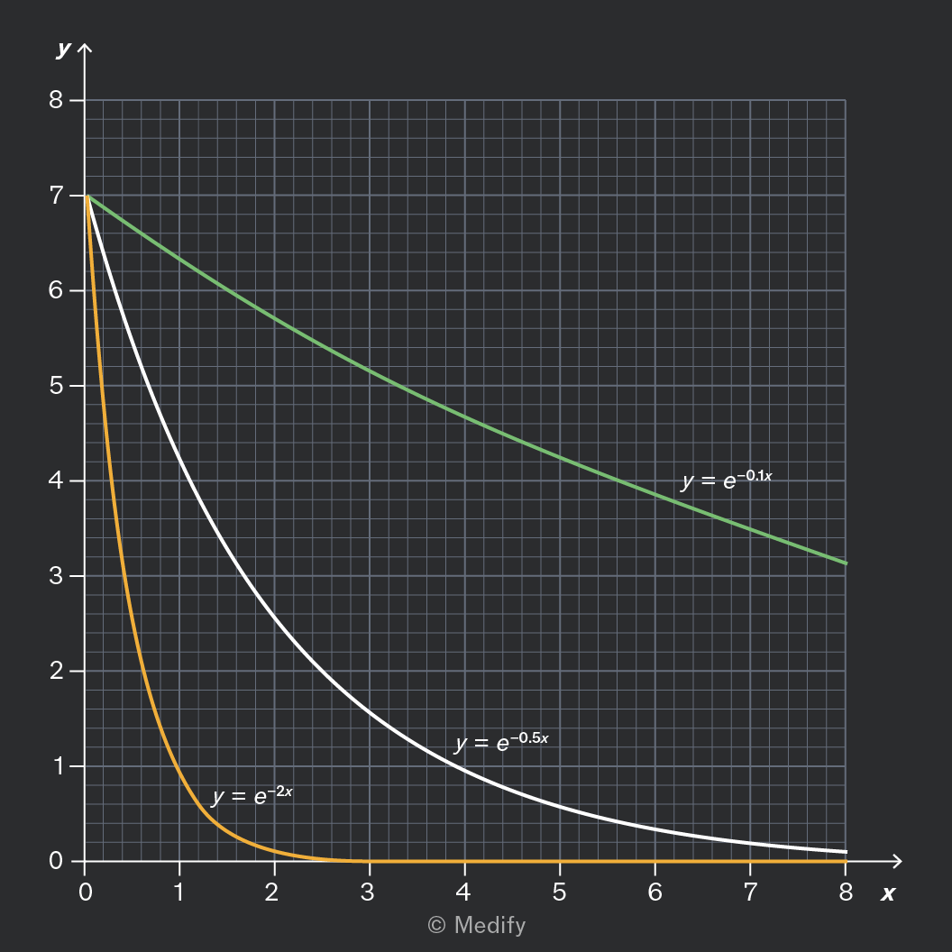
The decay constant appears in the equation for exponential decay:

It also appears in the rate equation – a related formula that describes decay:

It is useful to know that a larger decay constant means the decay is more rapid.
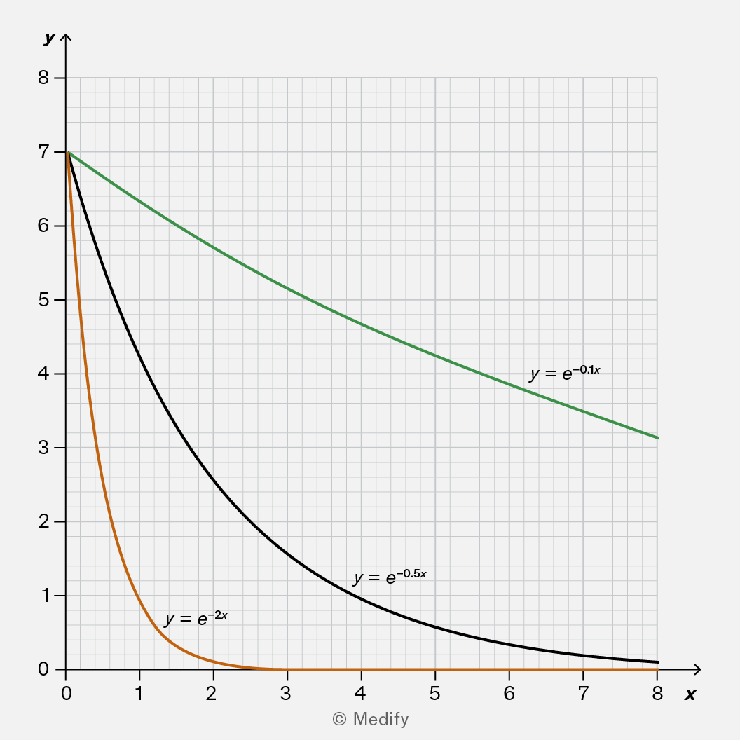
The image is a graph with a grid background, displaying three exponential decay curves labeled with equations. The x-axis is labeled 'x' and ranges from 0 to 8, and the y-axis is labeled 'y' and ranges from 0 to 8. There are tick marks at each integer value on both axes. The orange curve represents the function y = e^(-2x) and starts at approximately y=7 when x=0, rapidly decreasing to near y=0 by x=2. The black curve represents y = e^(-0.5x), starting at approximately y=7 when x=0, decreasing more slowly than the orange curve. The green curve represents y = e^(-0.1x), starting at approximately y=7 when x=0, and decreases the slowest among the three curves, remaining above y=3 at x=8. Each curve has its equation labeled next to it on the graph.

As you can see, these exponential curves have a similar shape. But the green curve with a decay constant of 0.1 decays very slowly. The orange curve with a decay constant of 2 decays much more rapidly.

Add to favourites

Question walkthrough

Apply understanding of exponential curves to solve a rate equation.

Uses the standard solution to an exponential decay rate equation to find the remaining mass of a radioactive isotope after a given time, using the initial mass to find the constant of integration.

You may encounter graphs where the vertical axis shows logarithms of a measurement. In some cases, the horizontal axis may also show logarithms. These are both logarithmic plots.

These graphs often show a straight line. However, this doesn’t mean they represent a linear relationship. You must not confuse them with a linear relationship.
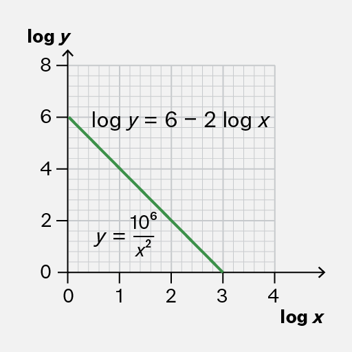
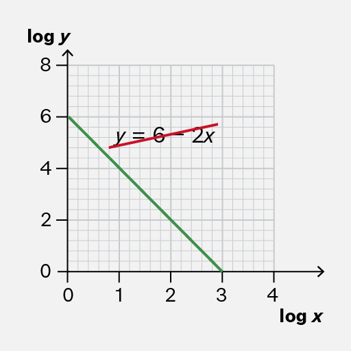
A graph with 'log y' as the vertical axis and 'log x' as the horizontal axis. The vertical axis ranges from 0 to 8, and the horizontal axis ranges from 0 to 4. A green line is drawn from approximately (0, 6) to (3, 0). Text annotations include 'log y = 6 - 2 log x' near the middle of the graph and 'y = 10^6 / x^2' below the line.
Do

Interpret logarithmic plots using logarithms as indicated.

It is useful to know that you can rearrange the equation to obtain an equation for in terms of

In this case,

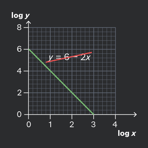
The image displays a graph with 'log y' as the vertical axis label and 'log x' as the horizontal axis label. The vertical axis ranges from 0 to 8, and the horizontal axis ranges from 0 to 4. There are two lines on the graph: a downward-sloping green line that starts at approximately (0, 6) and ends at (4, 0), and an upward-sloping red line near the top right, annotated with the equation 'y = 6 - 2x'.
Don't

Consider logarithmic graphs as showing linear (or proportional) relationships between data.

Add to favourites

You may need to interpret a semi-log graph, where the vertical axis shows a logarithm while the horizontal axis does not.

If this graph shows a straight line, this always indicates an exponential curve of the form where is the slope or gradient of the straight line.
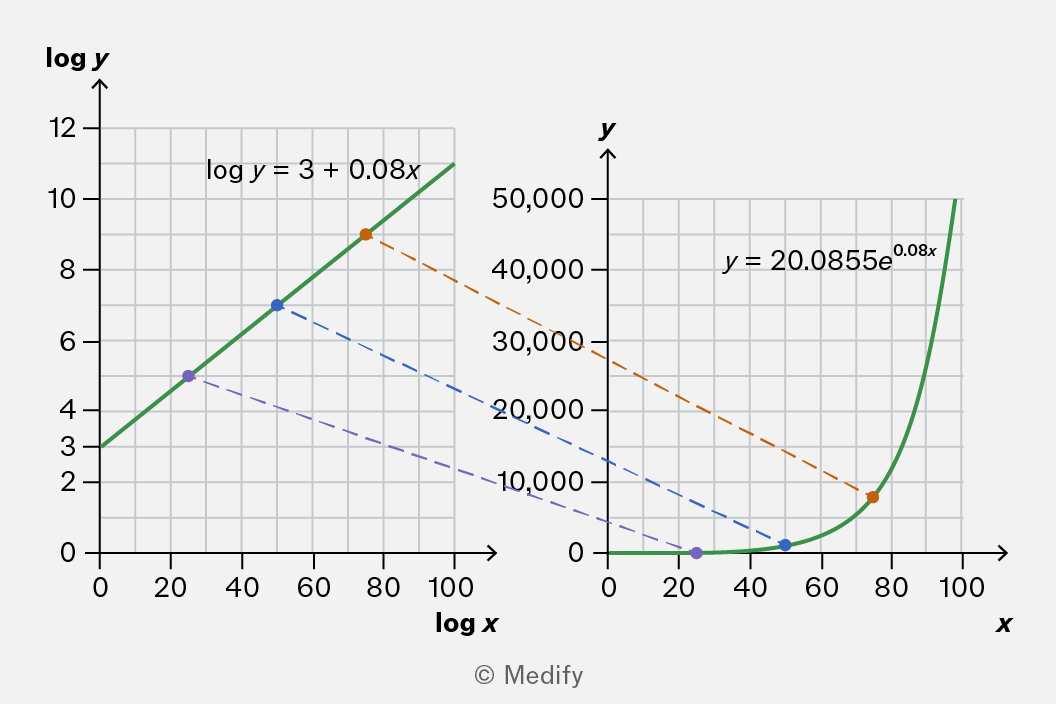
The image consists of two graphs side by side. The left graph has axes labeled 'log x' and 'log y'. The x-axis ranges from 0 to 100, and the y-axis ranges from 0 to 12. A green line represents the equation 'log y = 3 + 0.08x'. Three plotted markers are visible: approximately at (20, 5), (50, 7), and (80, 9), with an annotation 'log y = 3 + 0.08x' near the line. The right graph has axes labeled 'x' and 'y'. The x-axis ranges from 0 to 100, and the y-axis ranges from 0 to 50,000. A green curve represents the equation 'y = 20.0855e^0.08x'. Three plotted markers are visible: approximately at (20, 5000), (50, 10000), and (80, 30000), with an annotation 'y = 20.0855e^0.08x' near the curve. Dashed lines connect corresponding markers between the two graphs: orange for the highest values, blue for the middle values, and purple for the lowest values.

To see this, take the equation of the straight line, and take the exponent of both sides:

Add to favourites

You may need to interpret a log–log graph with both axes showing logarithms.

If the graph shows a straight line, this always indicates a power law of the form where is the slope or gradient of the straight line.
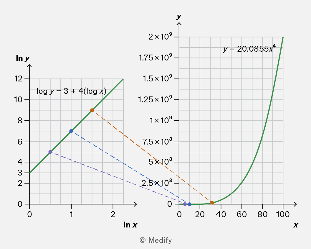
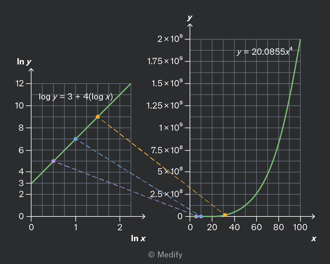
The image displays two graphs side by side. The left graph has 'ln y' on the y-axis and 'ln x' on the x-axis, with a linear plot labeled 'log y = 3 + 4(log x)'. The plot passes through points approximately at (0.5, 4), (1, 6), and (2, 9), marked by purple, blue, and orange dots respectively. The right graph has 'y' on the y-axis and 'x' on the x-axis, featuring a curve labeled 'y = 20.0855x^4'. The curve increases steeply, starting near the origin and rising sharply after x = 40. The right graph's y-axis has labels at intervals: 2.5×10^8, 5×10^8, 7.5×10^8, 1×10^9, 1.25×10^9, 1.5×10^9, 1.75×10^9, and 2×10^9. Dotted lines connect corresponding points between the two graphs.

To see this, take the equation of the straight line, and take the exponent of both sides:

Add to favourites

Question walkthrough

Determine an exponential relationship from a semi-log graph.

Uses a semi-log graph of a capacitor's discharge voltage to find the initial voltage and decay constant, then uses the decay constant and resistance to calculate the capacitance.

Question walkthrough

Determine a power law relationship from a log–log graph.

Uses a line of best fit on a log-log graph to find the gradient and intercept, then converts these into a power-law equation relating y and x.

The sine wave models many relationships in Physics, including circular motion and simple harmonic motion. You need to recognise the graph of and be aware of its key properties.
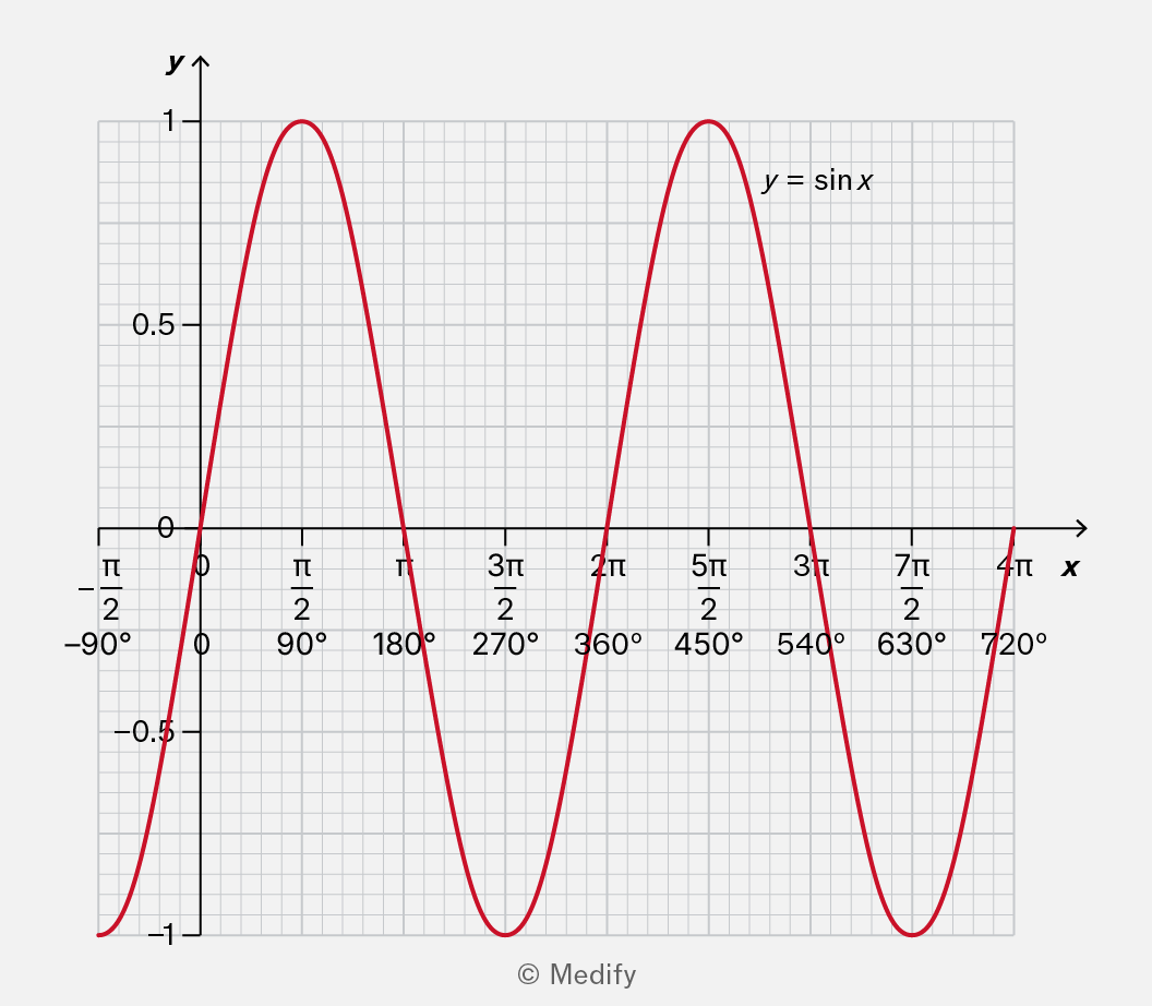
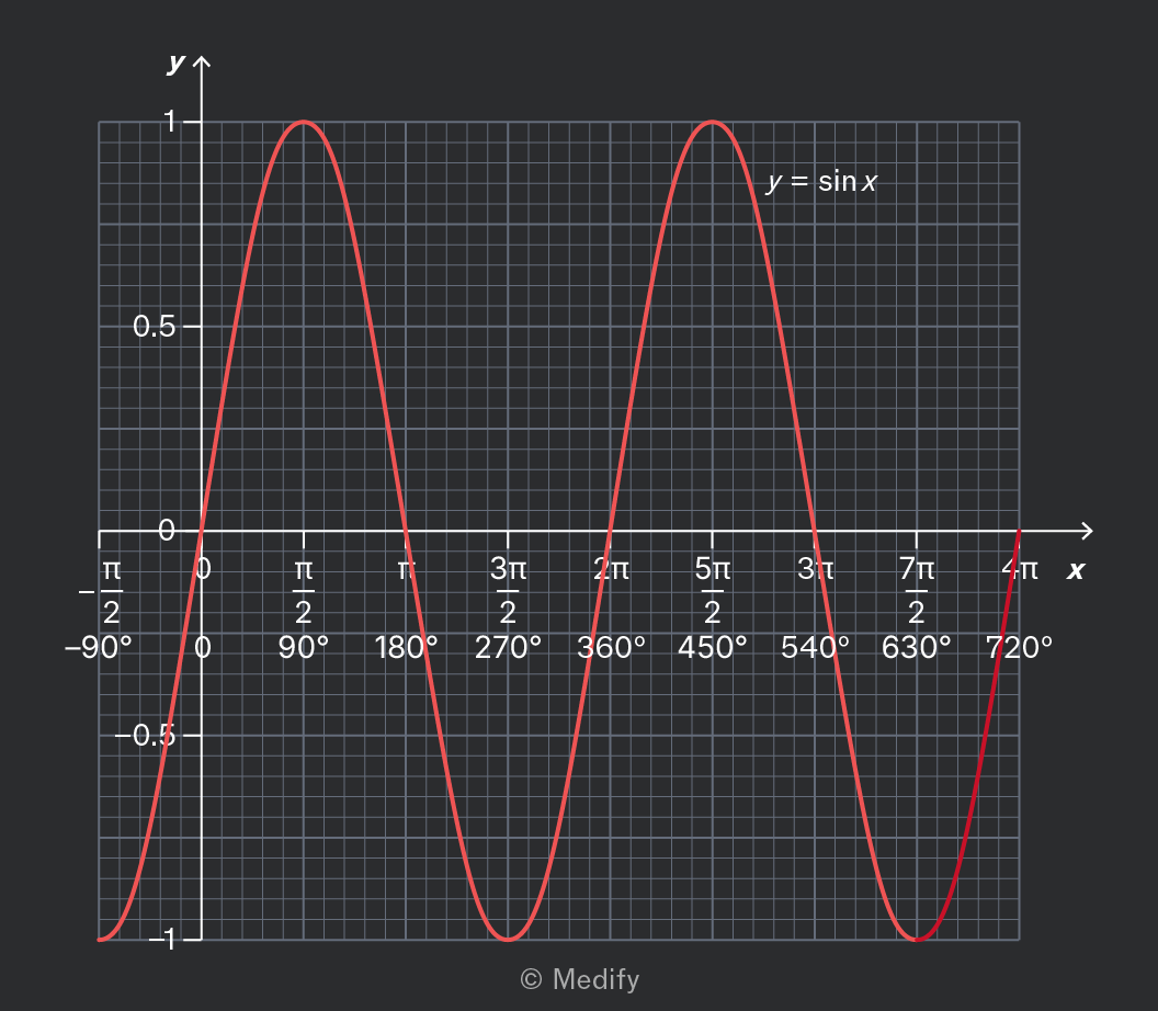
Graph of y = sin x with x-axis labeled from -90° to 720° and corresponding radian measures from -π/2 to 4π. The y-axis ranges from -1 to 1 with labels -1, -0.5, 0, 0.5, and 1. The sine wave starts at approximately -90°, reaches a peak at 90° (π/2), crosses zero at 180° (π), reaches a trough at 270° (3π/2), and completes two full cycles by 720° (4π). The graph includes grid lines and the function is plotted in red with the label y = sin x near the first peak.

It is important to note the following features of

  • Its maximum value is 1, and its minimum value is –1.
  • It passes through the origin; .
  • It is periodic (repeating every radians or 360 degrees).
  • It is odd (the negative part of the graph is the same as the positive part, but rotated).
Add to favourites

The sine wave models many relationships in Physics, including circular motion and simple harmonic motion. One form of the sine wave is the cosine, written as You need to recognise this graph and be aware of its key properties.
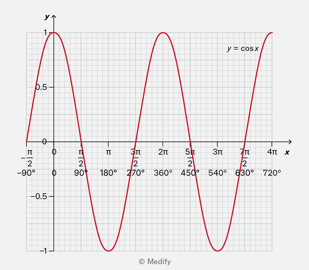
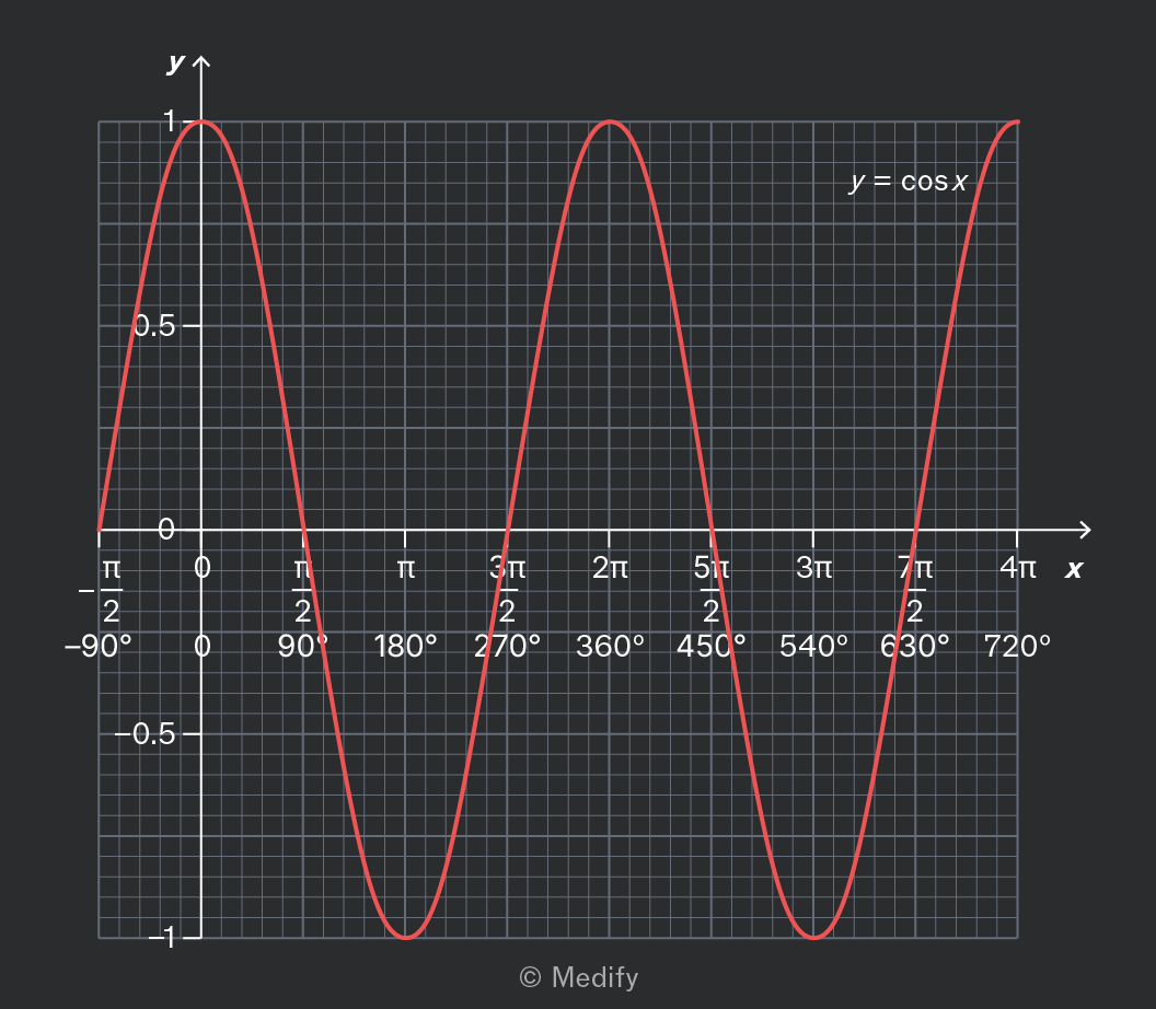
A graph displaying the cosine function y = cos x. The x-axis is labeled in radians and degrees, ranging from -π/2 (-90°) to 4π (720°). The y-axis is labeled with values from -1 to 1. A red curve represents the cosine function, starting at y=1 at x=0, reaching y=-1 at x=π, y=1 again at x=2π, and continuing the periodic pattern. The graph includes grid lines for reference. The label y = cos x is positioned near the first peak of the curve.

It is important to note the following features of

  • Its maximum value is 1, and its minimum value is –1.
  • It has its maximum value when In other words, .
  • It is periodic (repeating every radians or 360 degrees).
  • It is an even function (the negative part of the graph is the same as the positive part, but reflected).
Add to favourites

You will often encounter graphs of and Each of these is also a sine wave, but there are some key differences.
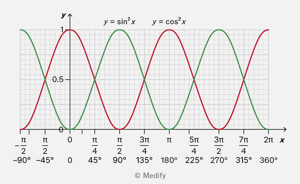
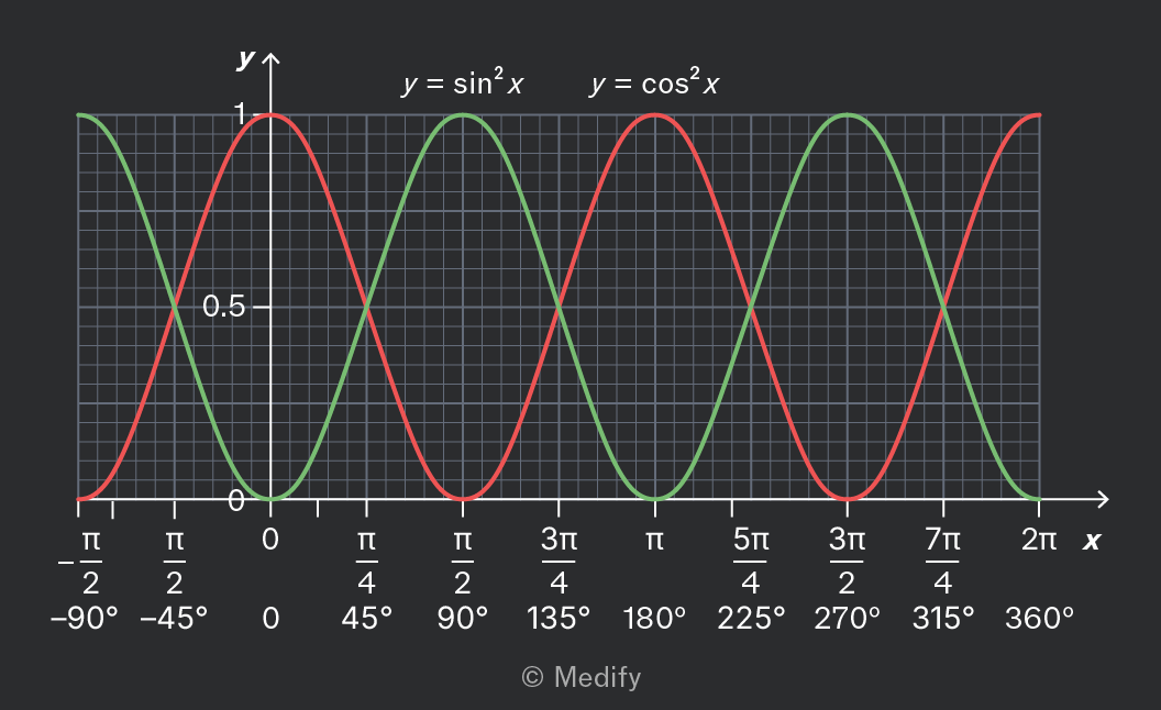
The graph shows two functions plotted on a grid with x and y axes. The x-axis is labeled with angles in both radians and degrees, ranging from -π/2 (-90°) to 2π (360°) with major grid lines at intervals of π/4 (45°), π/2 (90°), 3π/4 (135°), π (180°), 5π/4 (225°), 3π/2 (270°), 7π/4 (315°), and 2π (360°). The y-axis is labeled from 0 to 1 with a midpoint labeled at 0.5. A red curve represents y = sin²x and a green curve represents y = cos²x. Both curves oscillate between 0 and 1, with peaks at different x-values, showing the periodic nature of the functions. The label 'y = sin²x' is placed above the red curve, and 'y = cos²x' above the green curve.

It is important to note the following features of these graphs:

  • As the expressions are squared, they only take positive values, from a minimum of 0 to a maximum of 1.
  • passes through the origin like .
  • has its maximum value when like .
  • They are periodic, but with double the frequency, repeating every radians or 180 degrees. This is because the negative “half” of the wave becomes an extra (positive) wave.
  • and are even functions like . The negative part of the graph is the same as the positive part, but reflected.
Add to favourites

The tan graph is an important shape in physics and mathematics. You need to recognise the graph and be aware of its key properties.
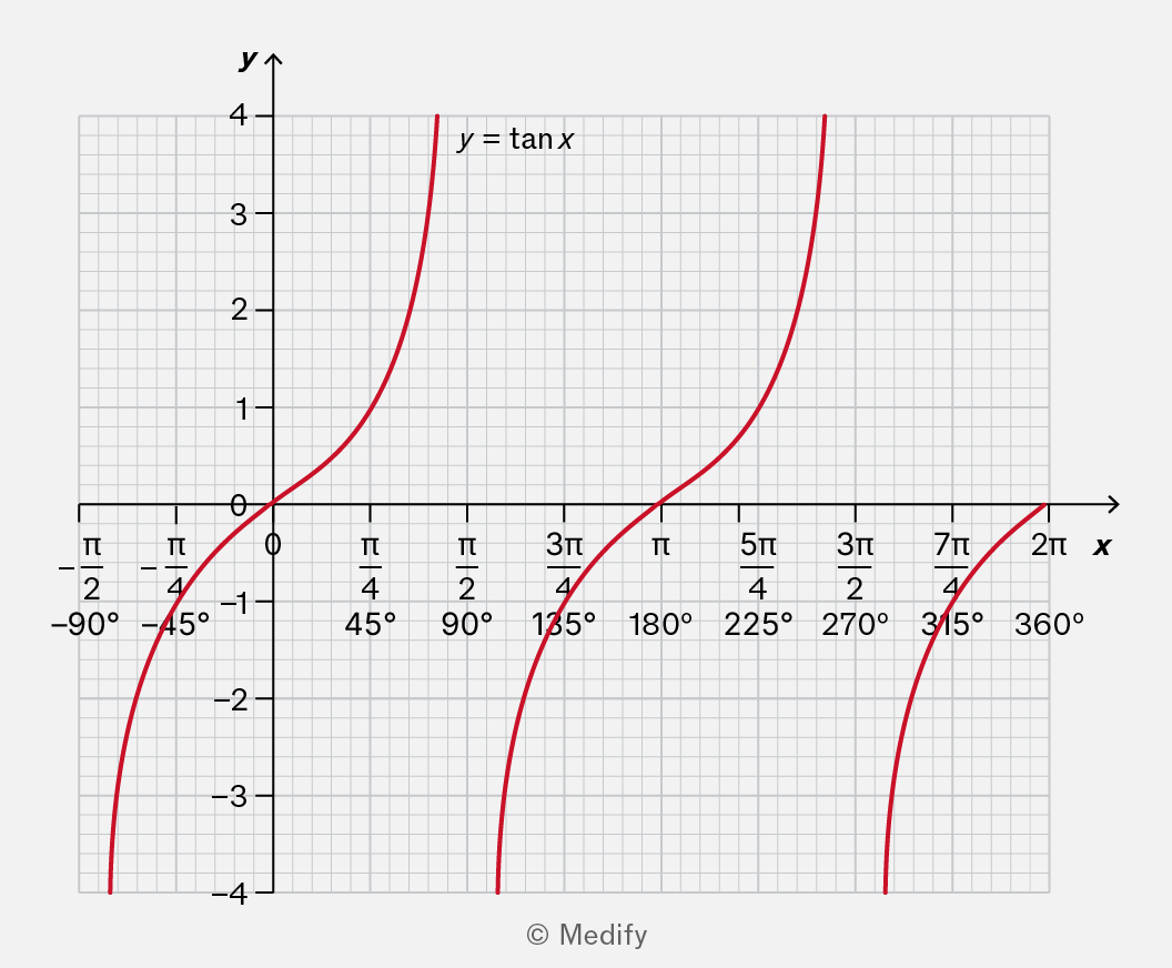
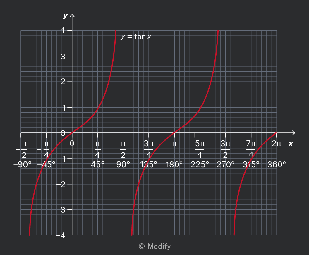
The image shows a graph of the function y = tan x. The x-axis is labeled with values in both radians and degrees: -π/2 (-90°), -π/4 (-45°), 0, π/4 (45°), π/2 (90°), 3π/4 (135°), π (180°), 5π/4 (225°), 3π/2 (270°), 7π/4 (315°), and 2π (360°). The y-axis is labeled with integer values from -4 to 4. The graph is a series of red curves representing the tangent function, with vertical asymptotes at x = -π/2, π/2, 3π/2, and so on. The curves approach infinity near these asymptotes. The annotation 'y = tan x' is placed near one of the curves.

It is important to note the following features of

  • It passes through the origin; .
  • It is periodic, repeating every radians or 180 degrees.
  • It is an odd function (the negative part of the graph is the same as the positive part, but rotated).
  • It has a vertical asymptote at etc. meaning that the graph becomes arbitrarily high or low as approaches these values.

It is useful to know that the vertical asymptote arises because a right-angled triangle with an adjacent side of length 1 could have an opposite side arbitrarily large. Another way to see this is using the identity:

When this fraction means a division by a number close to zero.

Add to favourites