Electromagnetism (6.3.3)

When a coil rotates within a magnetic field, the amount of flux passing through the coil will vary.

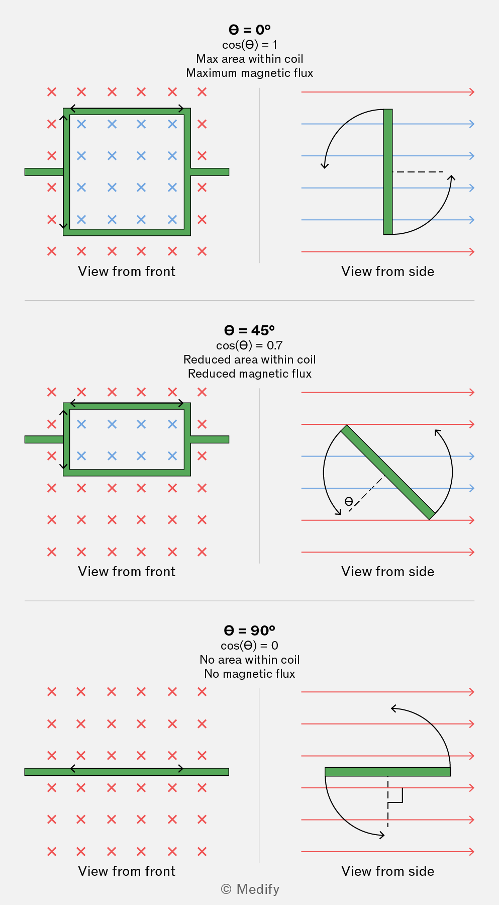
The diagram below shows the front and side views of a rotating coil. Blue field lines pass through the area within the coil, while red field lines do not.

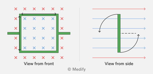
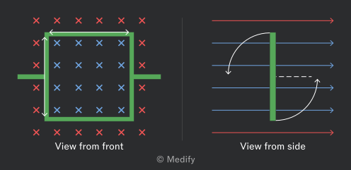
The crosses in the diagram above represent magnetic field lines coming from the page.

In this arrangement, the field lines are perpendicular to the plane of the coil. This means that at this moment in time, the magnetic flux is at its maximum as the area that the flux lines can pass through is greatest. The moment the coil rotates so the lines are no longer perpendicular, the magnetic flux will no longer be at its maximum.

The diagram below shows the front and side views of a coil resting in parallel to the magnetic field lines. This means that the magnetic flux will be zero, as the area through the coil that the flux lines can pass through is zero.

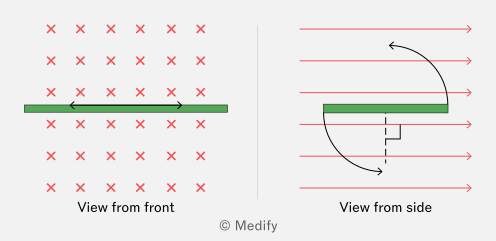
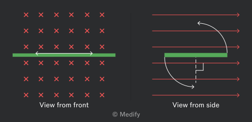
The crosses in the diagram above represent magnetic field lines coming from the page.

If the magnetic field lines are passing through an area at an angle between and , the magnetic flux can be calculated using:

Where:

• is the magnetic flux, it is measured in webers ,
• is the magnetic flux density, it is measured in teslas ,
• is the area, it is measured in meters squared and
• is the angle between the field lines and a line normal to the plane of the area, it is measured in degrees .

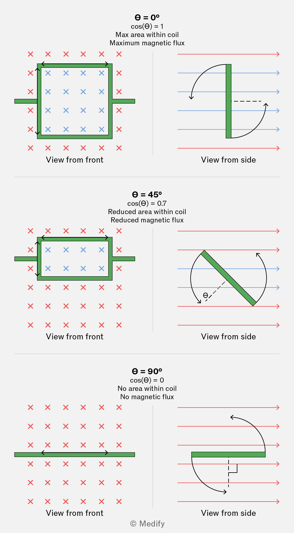
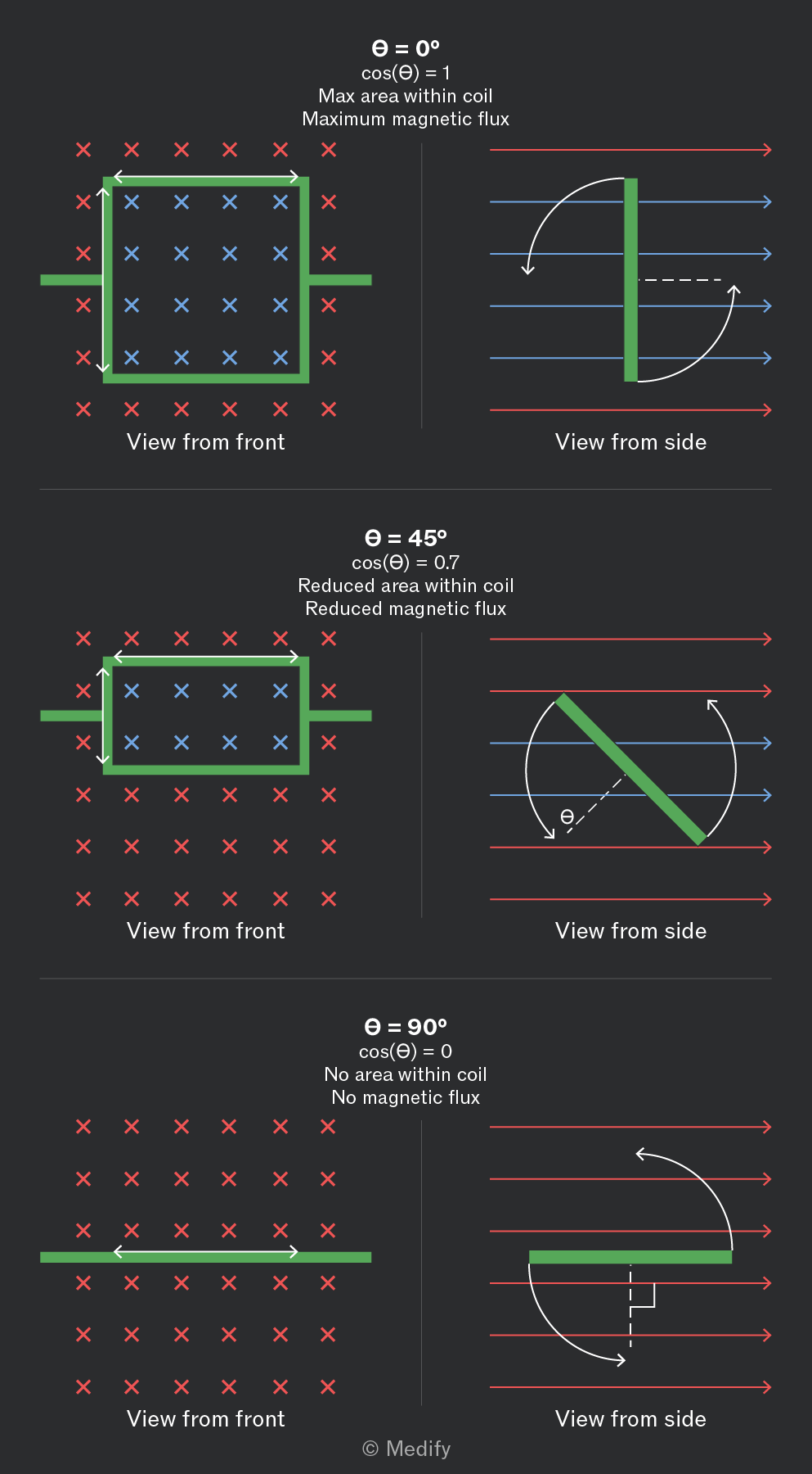
The diagram above shows a rotating coil in three different positions. The dashed black line represents the normal to the coil.

It is important to remember to use the angle between the field lines and this normal.

It is important to note that the magnetic flux linkage equals the magnetic flux passing through a coil multiplied by the coil’s number of turns. It can be found using the formula below:

Where:

• is the number of turns of the coil,
• is the magnetic flux, it is measured in webers ,
• is the magnetic flux density, it is measured in teslas , and
• is the area perpendicular to the magnetic field lines, it is measured in meters squared .

Flux linkage has units of weber turns turns.

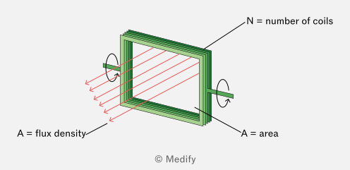
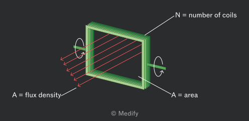
The magnetic flux lines passing through the coil may not be perpendicular to it. In this case, the following formula must be used to determine the magnetic flux linkage:

Where;

• is the number of turns of the coil.
• is the magnetic flux, which is measured in webers ,
• is the magnetic flux density, which is measured in teslas ,
• is the area, which is measured in meters squared and
• is the angle between the field lines and a line normal to the plane of the area, it is measured in degrees .

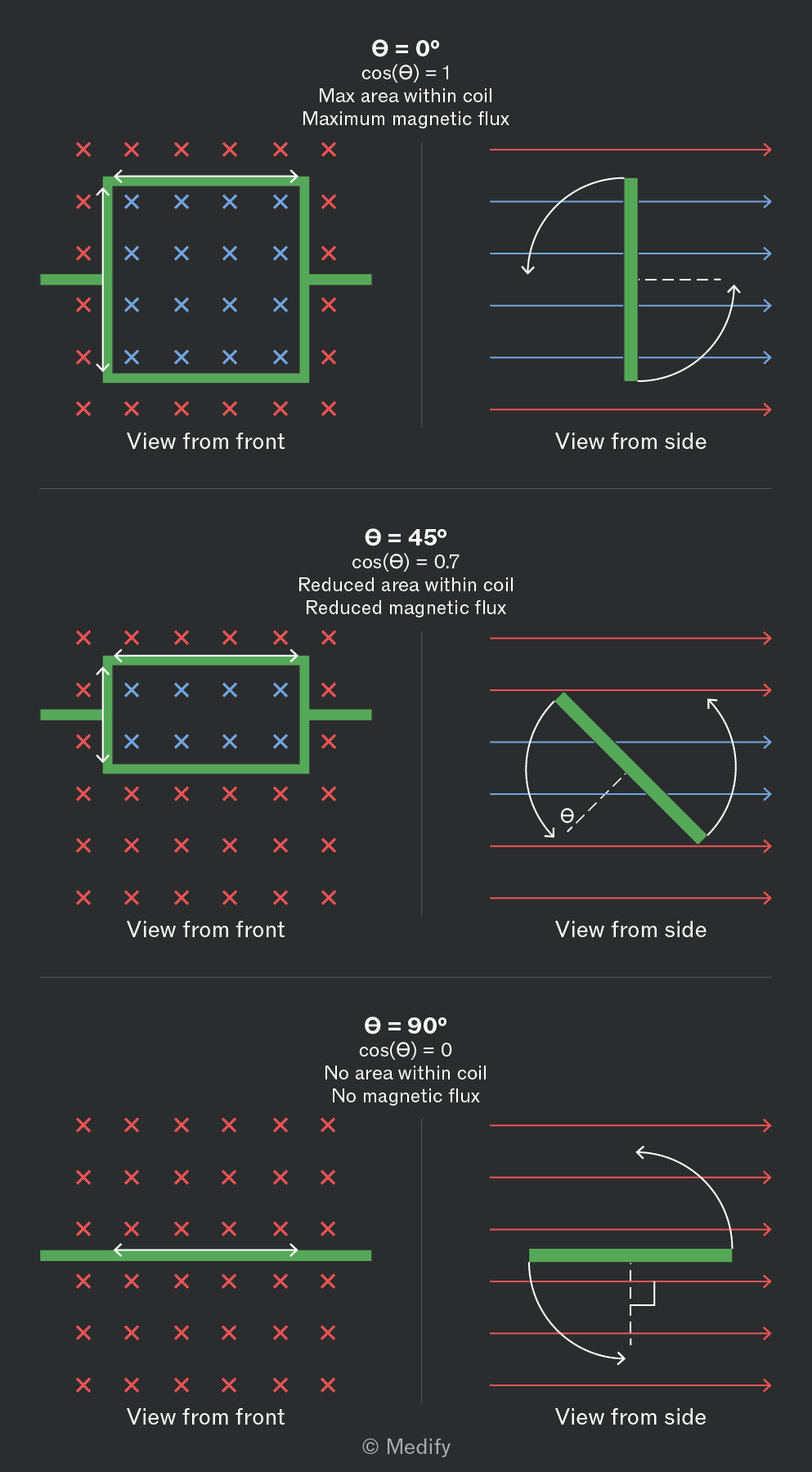
The diagram above shows a rotating coil in three different positions. The dashed black line represents the normal to the coil.

It is important to note that you should use the angle between the field lines and this normal in the magnetic flux linkage calculation.

The graph below shows how the magnetic flux linkage changes with time for a coil rotating within a magnetic field.

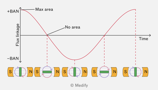
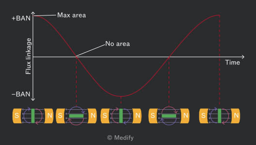
The flux lines pass from the magnet’s north pole to the magnet’s south pole. When the coil is upright (as shown on the far left), the area through which the flux lines can pass is at a maximum. This leads to the maximum flux linkage.

The graph follows a cosine curve to show how the flux linkage varies with time for a full rotation.

In a neutral wire, the charges are initially balanced. When the wire moves through a magnetic field, the Lorentz force acts differently on the free electrons (negative charges) than on the positive lattice ions. This force pushes the electrons to one side of the wire, creating a separation of charges. This separation sets up an electric field across the wire.

According to Fleming’s left-hand rule, the magnetic forces act differently on each end of the wire. The positively charged end experiences an upward force, while the negative charges in the opposite end are pushed downward.

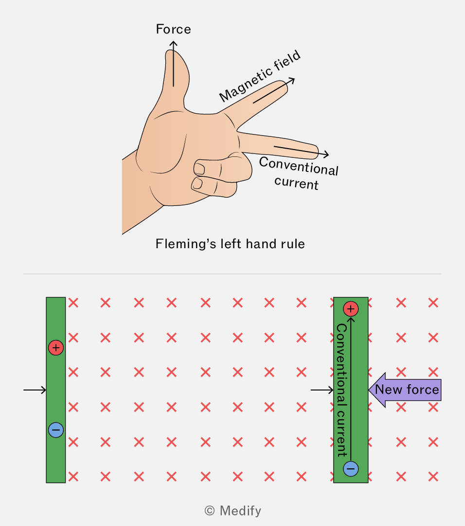
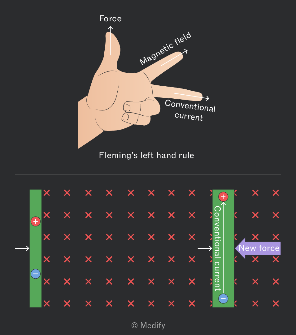
Since the conventional current is defined as the direction in which positive charges would flow, we say that the induced current flows upward in the wire. When we apply Fleming’s left-hand rule to this induced current, we see that it generates a magnetic force that opposes the original motion of the wire. This opposition illustrates Lenz’s law, which states that the induced EMF always acts to counter the change that produced it.

A scenario that demonstrates Lenz’s law is the movement of a permanent magnet towards a coil of wire connected to an ammeter. When the magnet is moved towards the coil, its magnetic flux lines move through the coil, causing a change in the magnetic flux. This, in turn, induces an EMF and, therefore, a current in the coil.

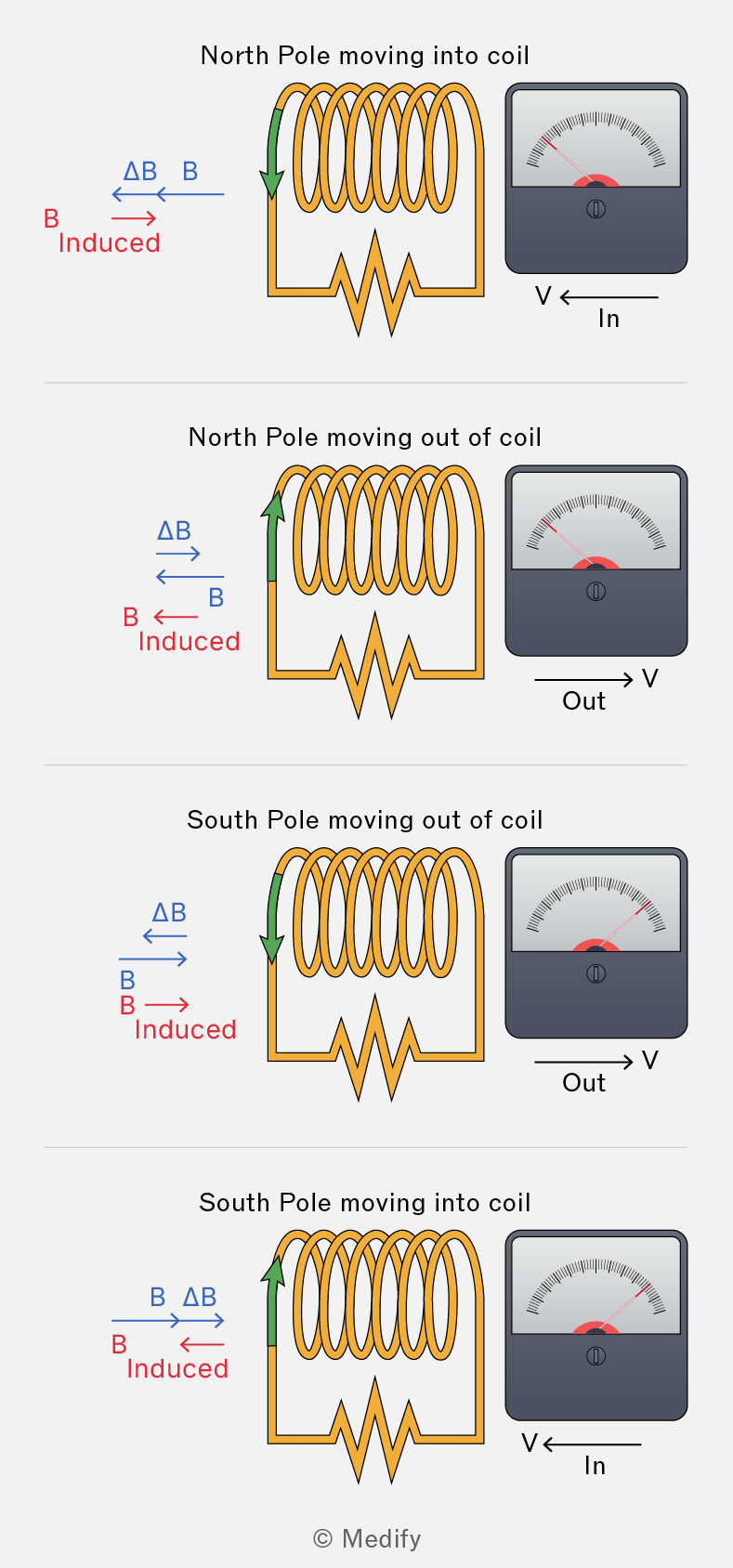
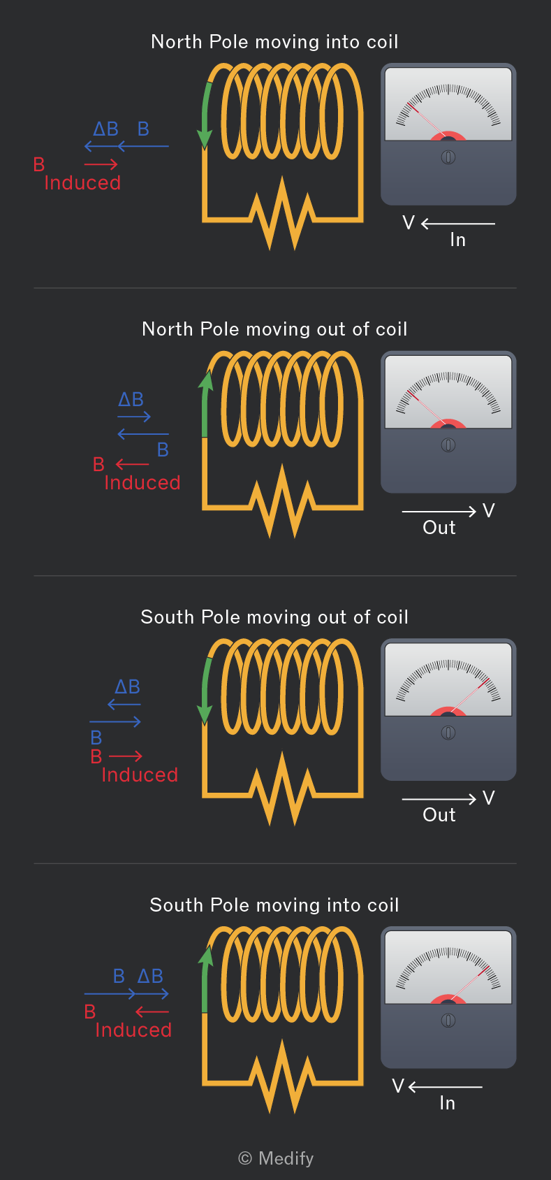
According to Lenz’s law, the induced EMF acts in such a direction as to oppose the change that caused it. In this scenario, as a magnet is moved into the coil, an EMF is induced, which induces a current.

The induced current in the coil will then induce a new magnetic field around it (according to Fleming’s right-hand rule). The magnetic field induced will be in a direction that opposes the magnet’s motion as it is moved towards it.

The EMF can be found from the gradient of a flux linkage against the time graph, as shown below. Please note that:

• if the gradient is positive, then the EMF will be negative,
• if the gradient is negative, then the EMF will be positive.

This is due to the inclusion of a negative sign in the Faraday equation due to Lenz’s law.

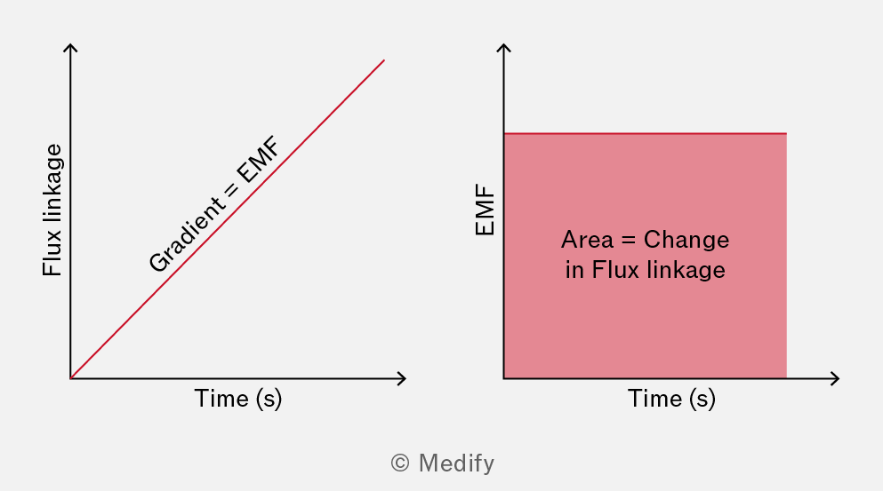
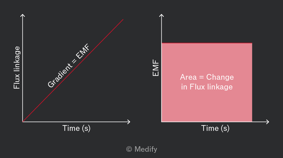
The change in flux linkage can be found from the area under an EMF against time graph.

As a coil rotates in a magnetic field, the flux linkage constantly changes due to the varying area within the coil that the flux can pass through.

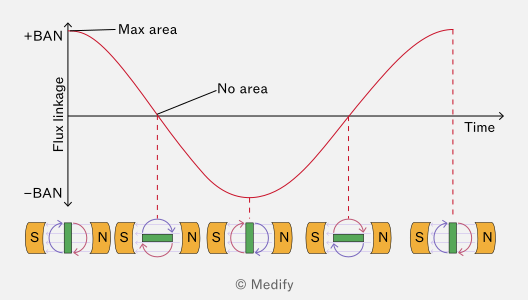
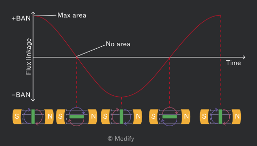
When the coil is perpendicular to the magnetic field lines, as shown on the far left of the graph above, the area within the coil that flux can pass through is at its greatest. Therefore, the flux linkage will be at its maximum.

When the coil is parallel with the magnetic field lines, the area within the coil which flux can pass is zero. Therefore, the flux linkage will also be zero and at its minimum.

Once the coil is rotated 180 degrees, as shown in the middle of the diagram, the area will once again be maximum, but as the coil is facing in the opposite direction, the polarity of the magnet has been reversed. Hence, the flux linkage is at a maximum but has a negative value.

The gradient of a flux linkage against time graph for a rotating coil in a magnetic field can be used to determine how EMF changes with time.

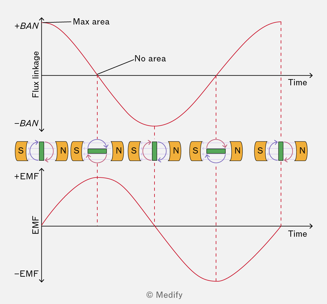
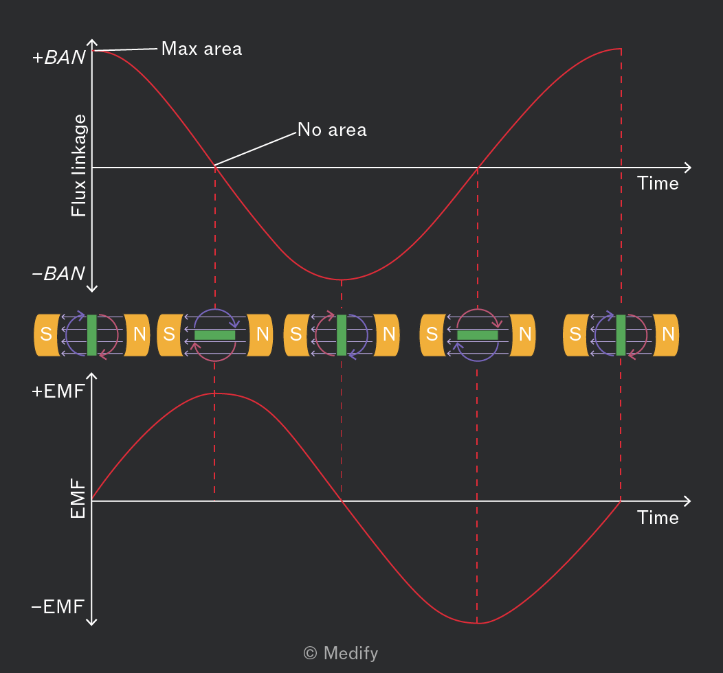
The graph of flux linkage against time and also the graph of EMF against time are both cosine, but with a phase difference of

It is important to note that for a rotating coil in a magnetic field, it might seem counterintuitive that the induced EMF is highest when the coil’s effective area – and thus its flux linkage – is smallest. However, EMF depends on the rate of change of magnetic flux, not just its magnitude.

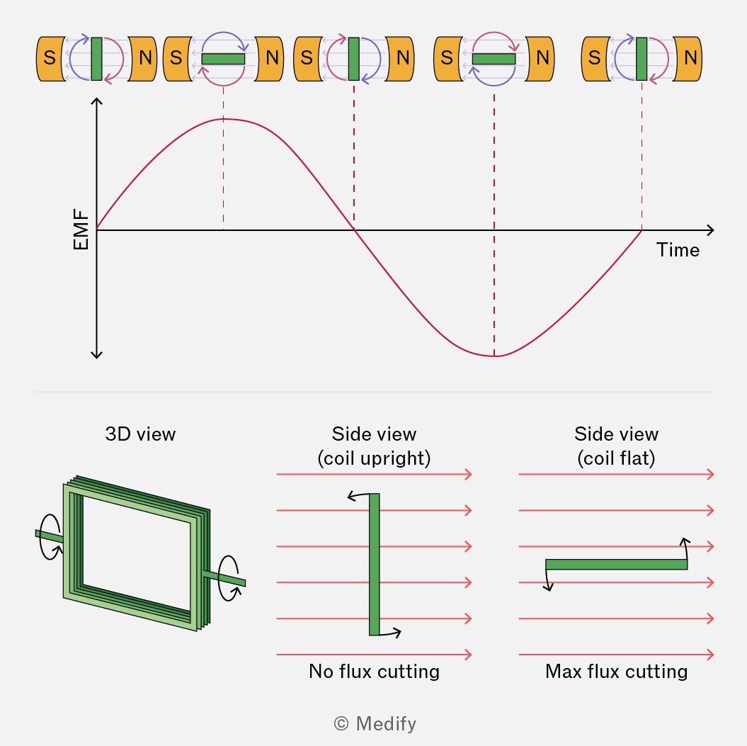
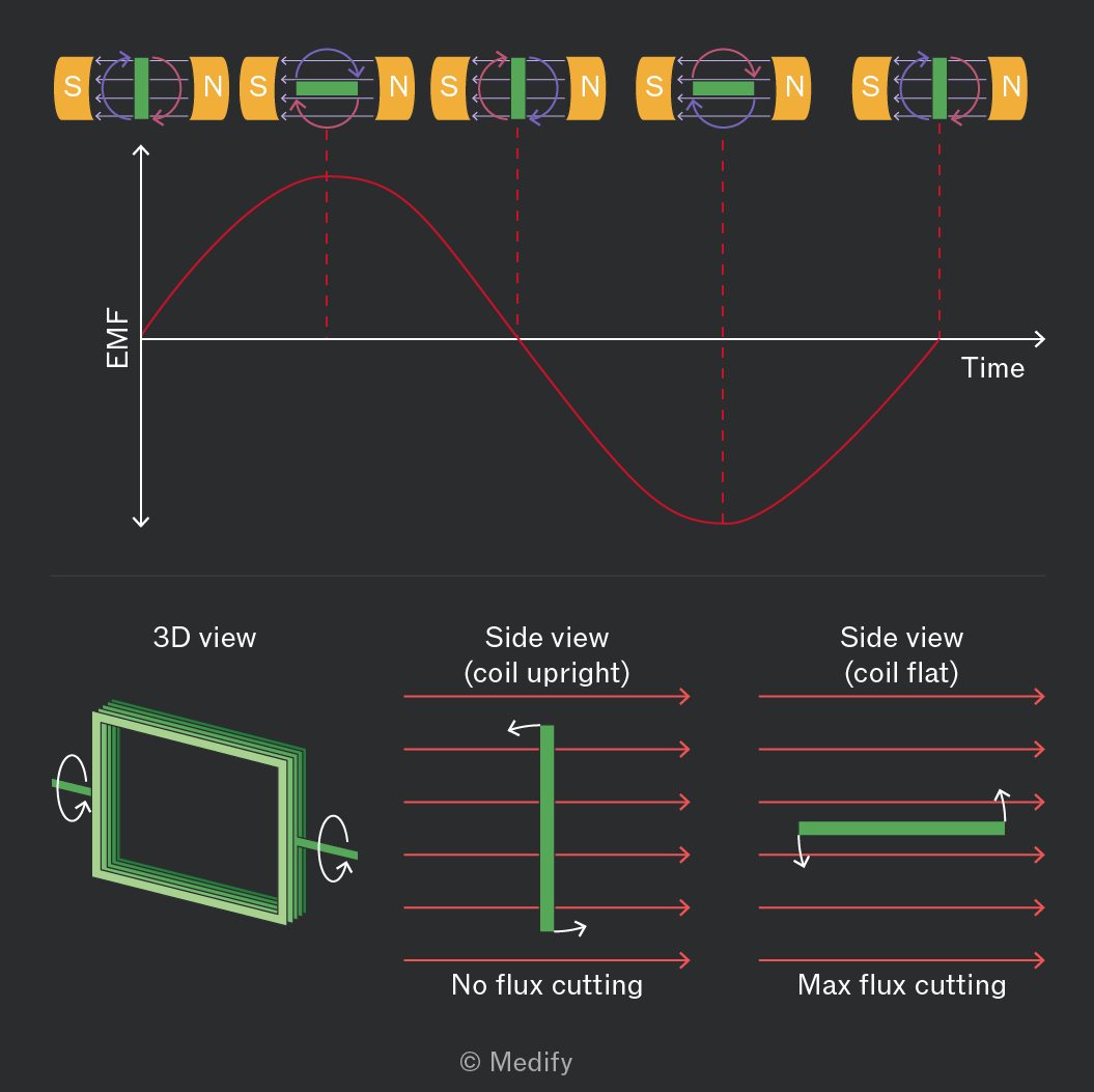
Only the top and bottom segments move when the coil is upright, travelling nearly parallel to the field lines, resulting in a slow change in flux and a low EMF. When the coil is flat, even a slight rotation causes these segments to rapidly cut through many field lines, producing a higher EMF according to Faraday’s law.

Thus, the induced EMF is more sensitive to the rate of flux change than to the absolute area exposed to the magnetic field.

A search coil can measure the alternating EMF created by a change in the magnetic flux.

In the diagram below, a coil of wire is connected to a signal generator, which produces an alternating current. This means that the coil is producing an alternating magnetic field.

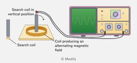
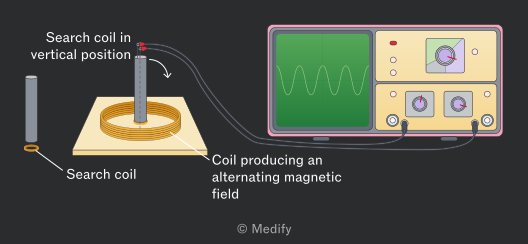
A second coil, known as a search coil, is placed within the first coil of wire. This coil will experience a continually changing magnetic flux, which will induce an EMF within it.

The alternating EMF can be measured directly if this search coil is connected to an oscilloscope.

An example of using a search coil is to carry out an experiment to investigate how the angle of the search coil affects the maximum EMF induced.

The search coil, a small coil of wire, is placed within a larger coil of wire, generating an alternating magnetic field. This alternating magnetic field will cause a change of flux linkage within the smaller coil, which in turn induces an EMF that can be measured.

The angle of this smaller coil can be adjusted, which will change the amount of flux linkage and the size of the maximum induced EMF.

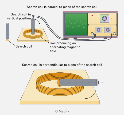
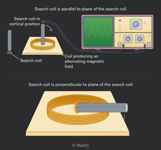
When the search coil is parallel to the plane of the first coil, it presents the greatest area for the changing magnetic flux to pass through. This means the greatest EMF will be induced.

When the search coil is rotated 90 degrees to be perpendicular to the plane of the first coil, it presents no area for the changing magnetic flux to pass through. This means no EMF will be induced.

To investigate how the angle of a search coil affects the maximum induced EMF, a small coil is placed inside a larger coil generating an alternating magnetic field. Changing the angle of the smaller coil alters the flux linkage, thereby affecting the maximum induced EMF.

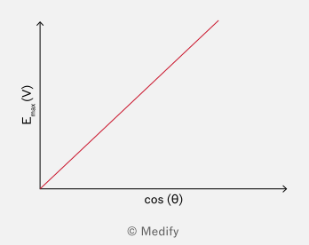
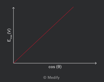
Then measure the max EMF induced for a range of angles between 0^o and 90^o and then plot a graph of the cosine of the angle between the planes of the two coils against max EMF. The result should be a straight line.

When a coil of wire is rotated in a magnetic field, a continual change in the magnetic flux linkage and EMF is induced. If the coil is part of a complete circuit, a current will also be induced.

A generator is a device in which an external force, such as a wind or steam turbine, rotates the coil.

There are two main types of generators used:

• alternators, which generate an alternating current (AC),
• dynamos, which generate a direct current (DC).

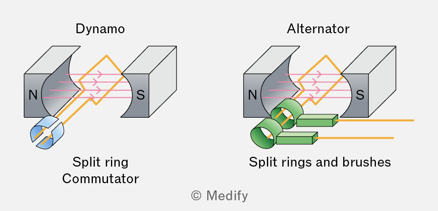
In an alternator, the rotating coil is attached to a series of slip rings and brushes. These allow the coil to maintain a constant connection to an exterior circuit even when it rotates.

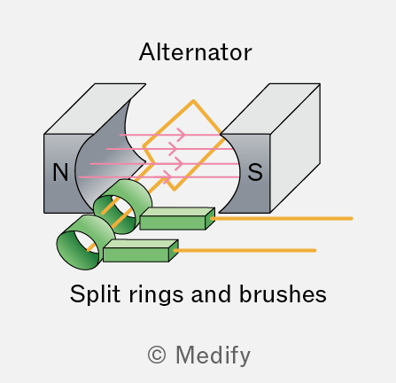
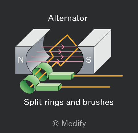
As the coil rotates, it causes a constant change in the magnetic flux, inducing an alternating EMF and, therefore, an alternating current in the coil.

A dynamo uses a setup similar to an alternator, except that instead of a series of slip rings and brushes it uses a split ring commutator.

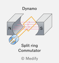
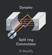
The split ring commutator does not allow a constant electrical connection between the coil and the external circuit.

The split ring commutator disconnects and reconnects the circuit every half turn. This keeps the current travelling in the same direction from the dynamo coil to the external circuit.

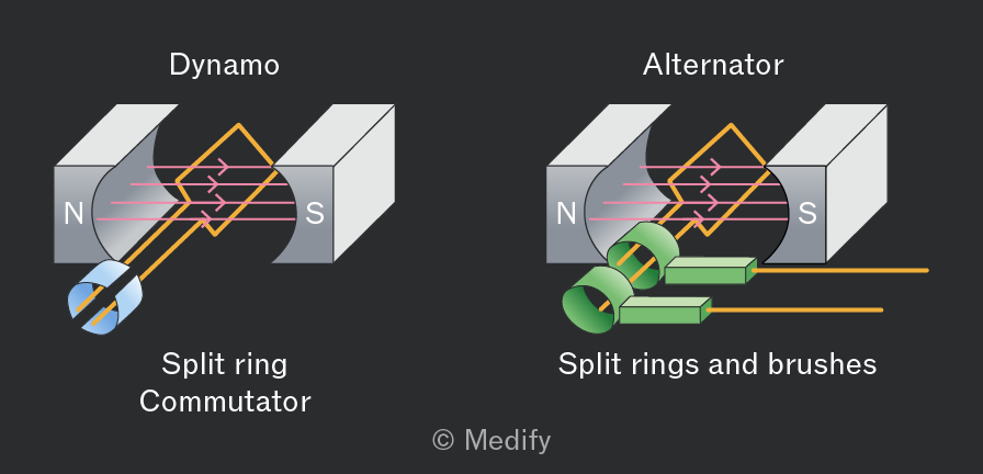
In an alternator, the rotating coil is attached to a series of slip rings and brushes. These allow the coil to maintain a constant connection to an exterior circuit even when it rotates. As the coil rotates, it causes a constant change in the magnetic flux, inducing an alternating EMF and, therefore, an alternating current in the coil.

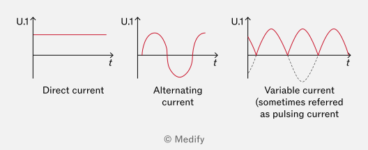
The split ring commutator used in a dynamo does not allow a constant electrical connection between the coil and the external circuit.

The split ring commutator disconnects and reconnects the circuit every half turn. This keeps the current travelling in the same direction from the dynamo coil to the external circuit, generating a variable current.

Transformers are devices designed to raise or lower the voltage in a circuit:

• A step-up transformer will raise the voltage and, at the same time, reduce the current.
• A step-down transformer will lower the voltage and increase the current.

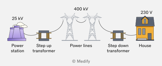
The national grid uses transformers to reduce the energy lost as heat in power lines. Since power is proportional to the current squared reducing the current by increasing the voltage helps reduce power loss and improve efficiency.

The transformer itself consists of three main components. A primary coil, a secondary coil and a soft iron core.

An alternating electric current is passed through the primary coil, creating an alternating magnetic field. The iron core helps to guide this magnetic field towards the secondary coil. The term soft describes how easily the iron core can be magnetized and demagnetized.

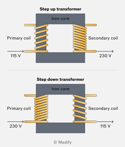
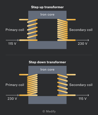
The secondary coil, therefore, experiences a continually changing magnetic flux linkage. According to Faraday’s law, this will induce an alternating EMF and current.

The magnitude of the EMF induced depends on the number of coils on the secondary coil. A step-up transformer will have more coils on the secondary coil to increase the voltage, whereas a step-down transformer will have fewer coils on the secondary coil to reduce the voltage.

An investigation can be conducted to prove the transformer equation experimentally and test the relationship between the number of coils and the current.

Start by wrapping a coil of wire around one end of an iron bar. Connect both ends of the wire to a power supply that can provide an alternating current. This is the primary coil. Use an ammeter in series with the power supply to accurately measure the generated current.

Wrap another coil of wire around the other end of the rod and attach another ammeter. This is your secondary coil.

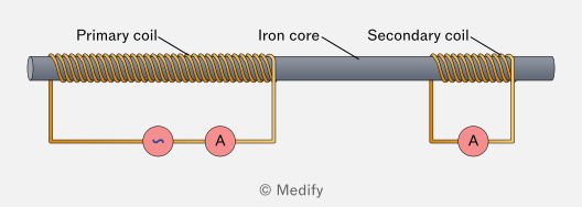
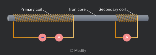
1. Count the number of coils in both the primary and secondary coils and record them in a table.
2. Turn on the power supply to provide an alternating EMF and record the current in the primary coil.
3. Record the current through the secondary coil and see whether the results collected obey the transformer equation:

Continue to test different combinations of current and coils and determine whether the equation continues to be obeyed. This equation assumes that the transformer is ideal and perfectly efficient and that 100% of the electrical power is transmitted from the primary to the secondary coil.

In reality, no transformer is 100% efficient. So, the results collected experimentally will not match what the equation predicts.