Foundations in physics

Foundations in physics introduces the core language and tools you’ll use throughout GAMSAT physics, from physical quantities and SI units to careful measurement, uncertainty, and error. It also builds the vector and scalar skills needed to interpret diagrams, resolve forces, and model motion and fields confidently.

14 min

Find only the order of magnitude ( etc.) of a physical quantity, or use approximations of known constants in calculations to provide numbers which are easier to work with. This technique can be used to quickly eliminate certain answer choices, or validate an answer obtained from a full calculation when reviewing your selected answer choices.

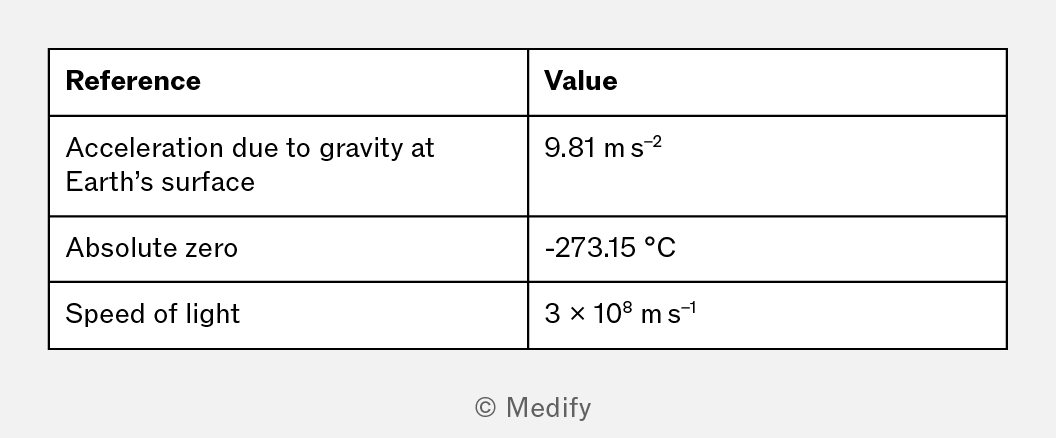
Some examples of commonly approximated constants are listed below:

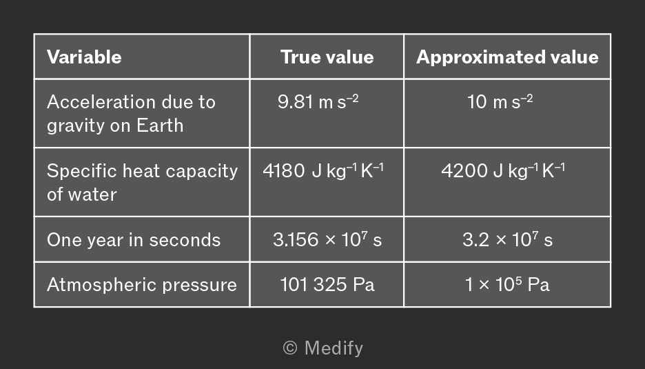
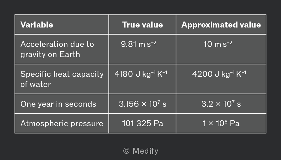
A table displaying various variables with their true and approximated values. The variables include: Acceleration due to gravity on Earth (True value: 9.81 m s−2, Approximated value: 10 m s−2), Specific heat capacity of water (True value: 4180 J kg−1 K−1, Approximated value: 4200 J kg−1 K−1), One year in seconds (True value: 3.156 × 10⁷ s, Approximated value: 3.2 × 10⁷ s), and Atmospheric pressure (True value: 101 325 Pa, Approximated value: 1 × 10⁵ Pa).

An example of an estimation calculation is determining the average weight of a person on Earth. Using Newton’s second law of motion, the force due to gravity acting on a person on the Earth’s surface is:

Where:

is the person’s mass, and
is the gravitational field strength.

Using and leads to:

Question walkthrough

Estimating Gravity on Mars from Force and Mass

Estimates the acceleration due to gravity on Mars by rounding an astronaut's mass and the force felt to convenient values before dividing.

The International System of Units (SI) is the standard set of units used by physicists and other scientists for measurements.

SI consists of seven quantities and their corresponding units, known as the SI base units, which are shown in the table below.

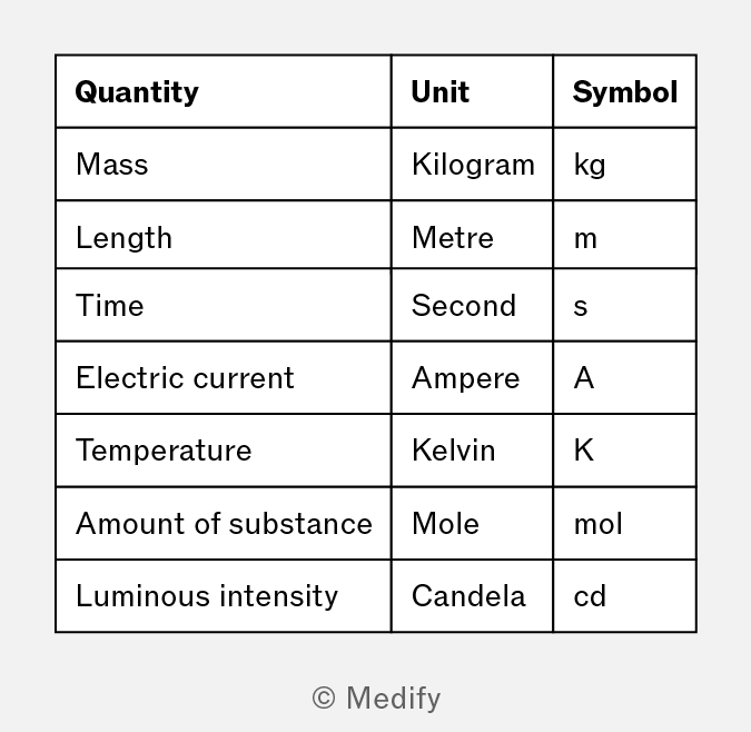
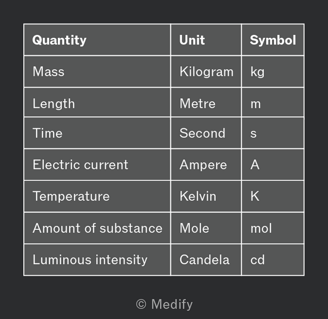
A table displaying various physical quantities, their units, and symbols. The quantities listed are: Mass (Kilogram, kg), Length (Metre, m), Time (Second, s), Electric current (Ampere, A), Temperature (Kelvin, K), Amount of substance (Mole, mol), and Luminous intensity (Candela, cd).

The SI base unit symbols are written in lowercase letters, except the symbols named after a person: kelvin has the symbol and the ampere has the symbol

There are many other physical quantities that can be measured, other than those corresponding to the SI base units.

Speed, acceleration, and force are examples of derived units. These quantities are known as derived quantities and are measured in derived units, which can be determined by substituting the base units into the equation that relates the derived quantity to the base quantities.

An example of this can be seen from the speed equation:

Where:

is speed,
is the distance travelled in a straight line, and
is the time taken.

Substituting the base units for length and time leads to:

Many derived units are used so frequently in measurements that they have been given specific names. A few of the most useful derived units are shown in the table below.

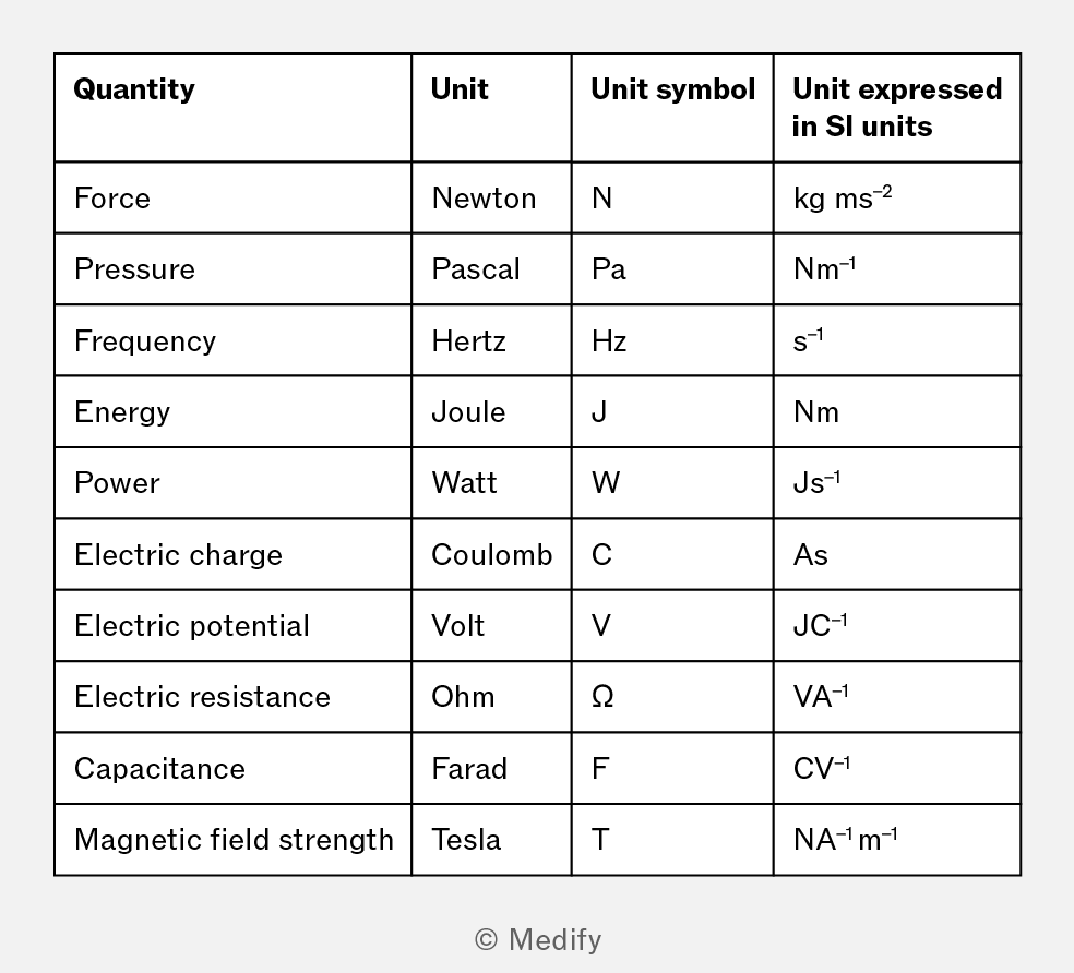
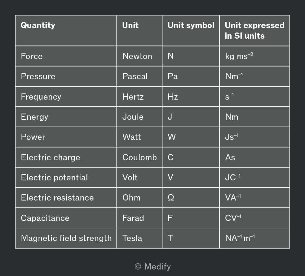
A table displaying various physical quantities along with their units, unit symbols, and units expressed in SI units. The quantities listed are Force (Newton, N, kg ms²), Pressure (Pascal, Pa, Nm⁻¹), Frequency (Hertz, Hz, s⁻¹), Energy (Joule, J, Nm), Power (Watt, W, Js⁻¹), Electric charge (Coulomb, C, As), Electric potential (Volt, V, JC⁻¹), Electric resistance (Ohm, Ω, VA⁻¹), Capacitance (Farad, F, CV⁻¹), and Magnetic field strength (Tesla, T, NA⁻¹m⁻¹). The table is attributed to Medify.

It is useful to note that it is much more convenient to use these abbreviated units rather than write out the full SI units during calculations. All of the above units are capitalised since they are named after people.

Physical equations must have the same units on either side: in other words, they must be homogeneous. The homogeneity of a physical equation can be checked by substituting SI base units into either side of the equation to ensure that both sides result in the same combination of SI units.

An example of this can be demonstrated with an equation of motion for uniform acceleration:

Velocity on the LHS of the equation has SI base units of For on the RHS, SI base units must be substituted for initial velocity , acceleration and time

It is important to note that the numerical coefficient of 2 is dropped, as pure numbers are dimensionless. The equation is homogeneous:

Prefixes are used to represent decimal submultiples or multiples of SI units in compact form.

For example:,

can instead be written as and
is equal to

A list of the most useful prefixes required for your exams is shown in the table below.

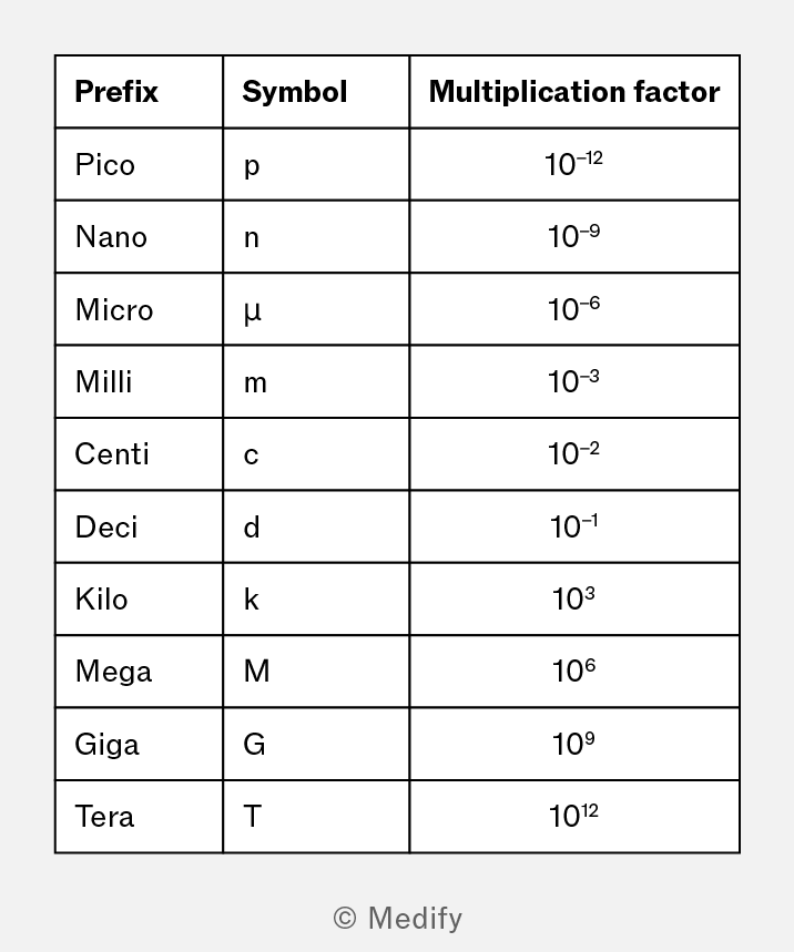
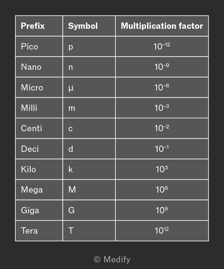
A table displaying metric prefixes, their symbols, and multiplication factors. The prefixes listed are Pico (p), Nano (n), Micro (μ), Milli (m), Centi (c), Deci (d), Kilo (k), Mega (M), Giga (G), and Tera (T) with corresponding multiplication factors of 10^-12, 10^-9, 10^-6, 10^-3, 10^-2, 10^-1, 10^3, 10^6, 10^9, and 10^12 respectively. The table is attributed to Medify.

All the prefixes with a multiplication factor greater than one are in uppercase, with the exception of kilo, whereas all the prefixes with a multiplication factor less than one are in lowercase.

The error of a measurement is the difference between an individual measurement and the true value of the quantity being measured. There are two types of errors, random and systematic.

Random error results in a random fluctuation of the measured value about the true value over repeated measurements.

Examples of causes of random error include:

Fluctuations in the external conditions, such as electronic noise in an electrical component.
Reading the measuring instrument differently each time, such as the level of the line on a thermometer.

Random error is often unavoidable, but its effect can be reduced by using more precise measuring instruments or taking many repeated measurements and averaging them to find the mean value.

Systematic error results in a skewing of the measured data by a given amount related to a flaw in the measurement process. Systematic errors can be reduced by calibrating the measurement apparatus or by comparing the results of different measurement techniques if possible.

Examples of systematic error include:

Zero error – caused by the measuring instrument not being calibrated correctly, such as a weight scale showing a non-zero reading when no object is placed on it.
Scale error – when measurements are consistently different from the true value by a certain proportion. For example, a weight scale may measure higher than the true value.

Random errors, where all results are affected by fluctuating amounts, affect the precision of a measurement, which describes the closeness of independent test results made under the same conditions. Precision depends only on the distribution of the random errors about the true value and does not depend on the true value itself.

Systematic errors, however, skew all results by a consistent amount and impact the accuracy of a measurement. Accuracy reflects how closely an individual test result aligns with the true value.

Sometimes, an accepted reference value can be used as the true value; however, the true value is usually unknown and must be measured.

A table with two columns titled 'Reference' and 'Value'. The rows include: 'Acceleration due to gravity at Earth’s surface' with a value of '9.81 ms²', 'Absolute zero' with a value of '-273.15 °C', and 'Speed of light' with a value of '3 × 10⁸ m s⁻¹'.

The way that systematic and random errors affect accuracy and precision can be visualised by imagining a person throwing darts at a dartboard.

In the left image, the darts land near the bullseye with a random spread. This is an example of random error. The dart throws are both precise and accurate.

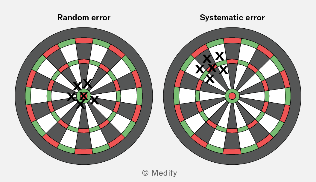
Left dartboard labeled 'Random error' with a cluster of marks near the center, and right dartboard labeled 'Systematic error' with marks clustered in one area.

Systematic error in dart throwing in the right image causes a consistent deviation from the intended target, causing darts to consistently land in a particular area off-centre, rather than being randomly scattered. It’s often caused by a flawed technique, such as an improper grip, a poor follow-through, or an incorrect stance, which biases the throws in a predictable direction.

The darts will have a similar spread, but their average position will be displaced from the centre of the bullseye. This is an example of systematic error. The dart throws are precise but not accurate.

Uncertainty is an estimate attached to a measurement which characterises the range of values which should contain the true value.

When using analogue measurement tools with a graduated scale that can be read, the uncertainty is taken as half of the smallest graduation. For example, a ruler with divisions of has an absolute uncertainty of

When using a digital apparatus, the uncertainty is equal to the smallest graduation. For example, a one decimal place ammeter has an absolute uncertainty of

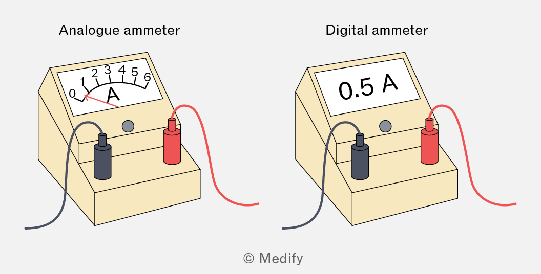
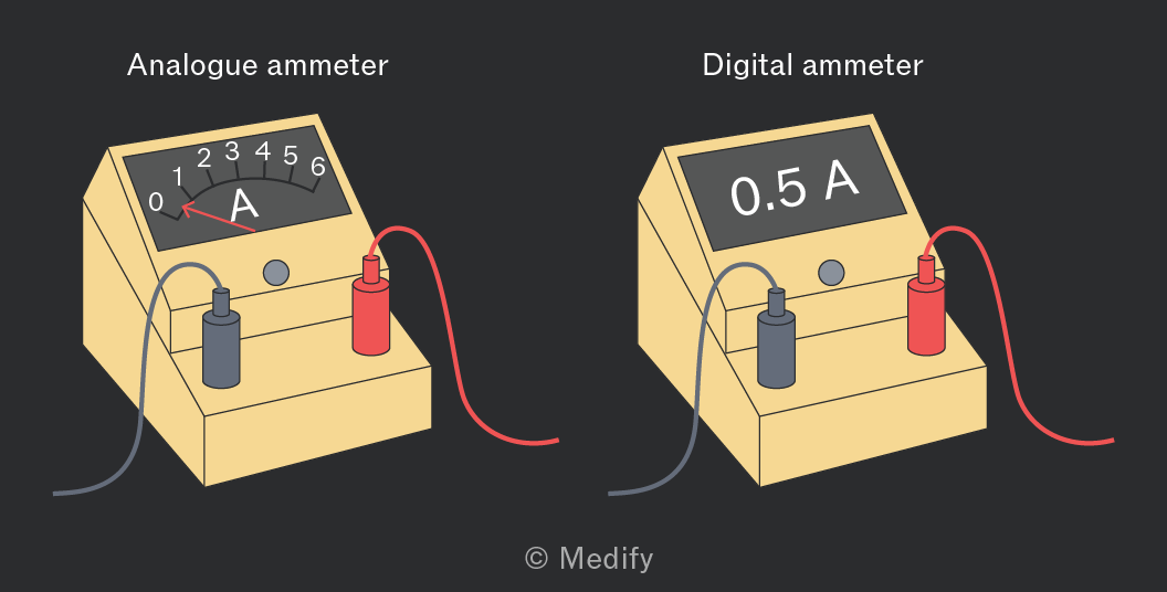
Analogue ammeter showing a needle pointing to A on a scale from 0 to 6, and a digital ammeter displaying 0.5 A.

Percentage uncertainty is the ratio of the absolute uncertainty to the quantity measured as a percentage, which can be written as:

For example, if a ruler with absolute uncertainty is used to measure a length of the percentage uncertainty is:

When multiple measurements are combined, the uncertainty in the final result will be a combination of the uncertainties in each measurement. So, when measurements are added or subtracted, the absolute uncertainties are summed.

An example of absolute uncertainty is in finding the tensile strain of a metal bar by measuring the change in length before and after the application of force.

If the initial length is and the final length is then the change in length is:

The uncertainty is:

So the change in length is:

When measurements are multiplied or divided, the percentage uncertainties must be added.

An example of percentage uncertainty is the calculated resistance of a resistor. It is found by measuring the current, for an applied voltage, .

The percentage uncertainty in and respectively is:

Ohm’s law can be rearranged to:

This expression shows that the percentage uncertainty in is found by adding the percentage uncertainties in and . Therefore, the percentage uncertainty in is:

Raising to a power is a special case of multiplication. The percentage uncertainty is multiplied by the power to which the value is being raised.

For example, consider measuring the power supplied to a resistor of resistance with current flowing through it. The percentage error in is and the percentage error in is

Electrical power, is given by:

Therefore, the power through the resistor is:

The percentage uncertainty in the power is equal to twice the percentage uncertainty in since it is raised to the power of two, added to the percentage uncertainty in which is:

Therefore, the uncertainty in the power is:

The calculated power is written as:

Each data point, based on a measured value, has an associated uncertainty. Error bars are a way to visually represent this uncertainty. They are drawn stretching above and below the data point by the absolute uncertainty in each direction. If there are no horizontal or vertical error bars for a data point, then the error is negligible in the X axis or Y axis measurement.

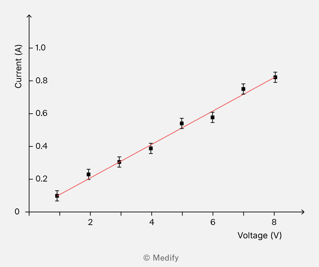
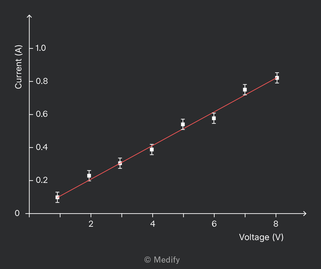
A graph showing Current (A) on the vertical axis and Voltage (V) on the horizontal axis. The graph includes data points with error bars and a red line indicating the trend. The vertical axis ranges from 0 to 1.0 A, and the horizontal axis ranges from 0 to 8 V.

Error bars can be used to find anomalous data points. If an error bar does not pass through the line of best fit and is a significant distance away from it, the data point is likely an anomaly.

Error bars can be used to estimate the uncertainty in the gradient of the line of best fit, which can be done by drawing the worst lines of fit. These lines are drawn from the bottom of the first error bar to the top of the last error bar and vice versa.

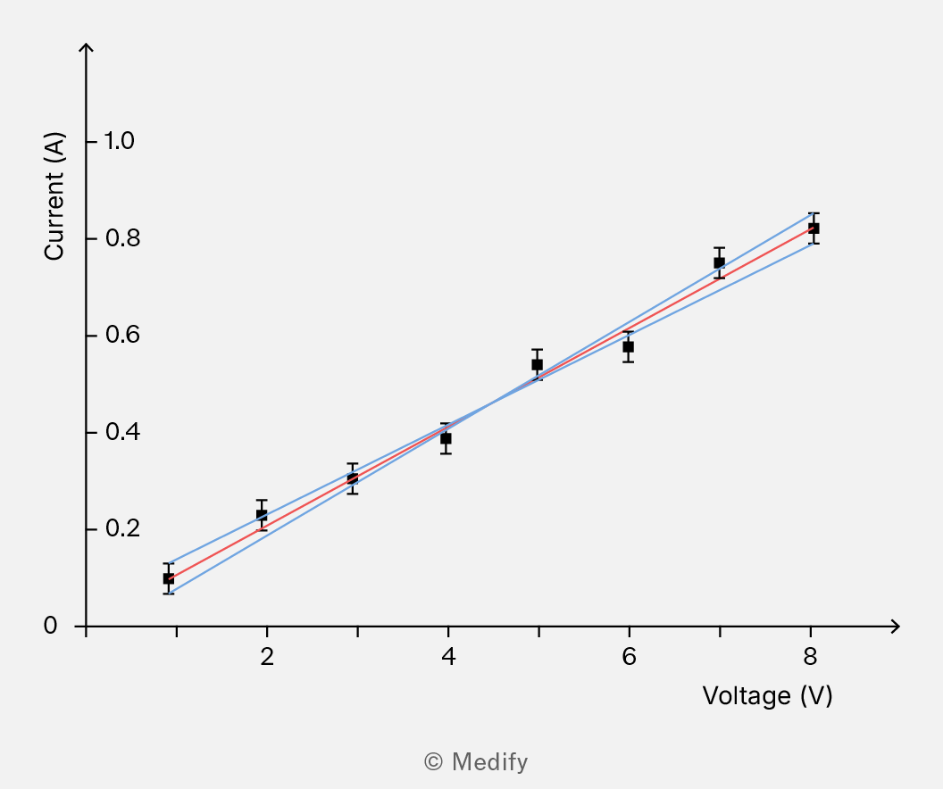
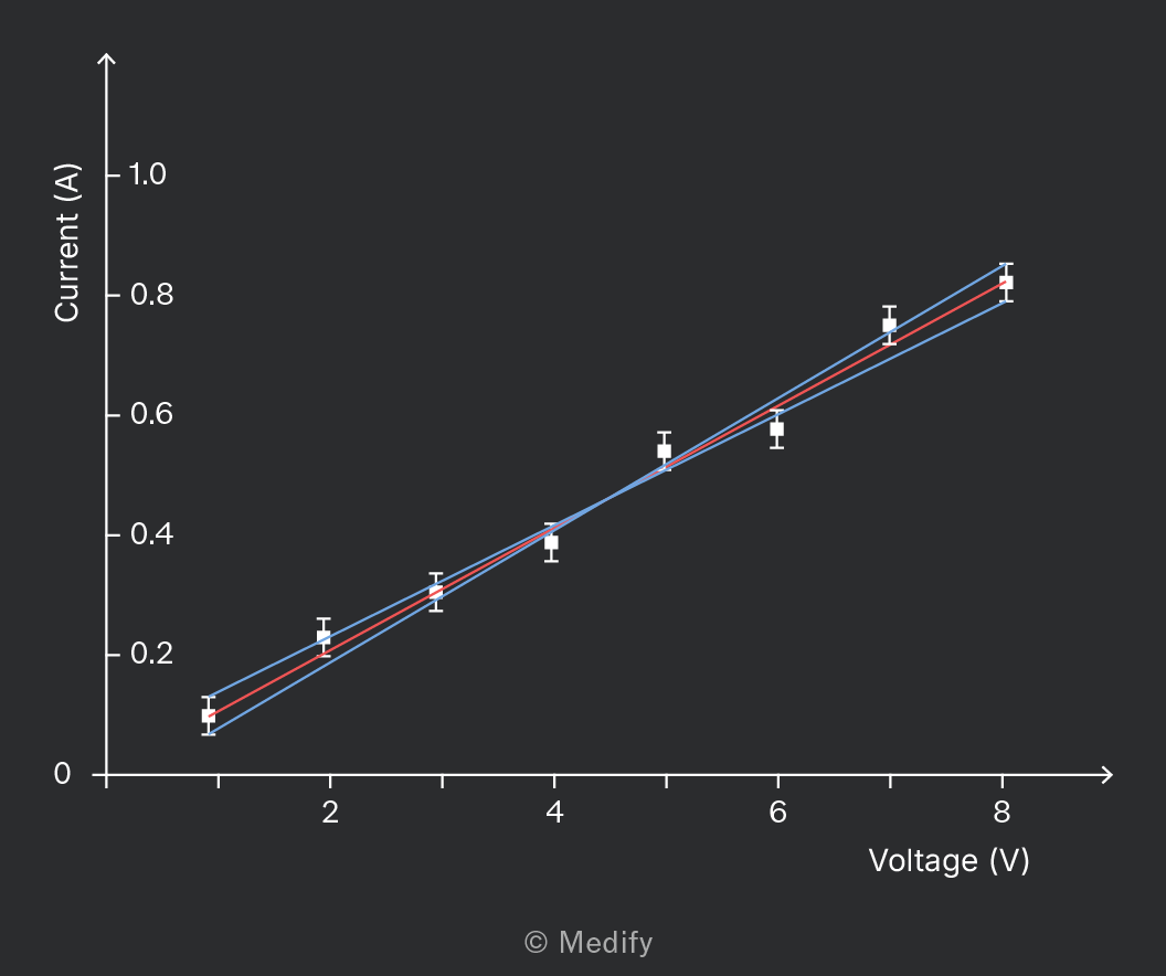
A graph showing Current (A) on the vertical axis and Voltage (V) on the horizontal axis. The graph includes data points with error bars, and two lines representing different datasets, one in blue and one in red. The current values range from 0 to 1.0 A, and the voltage values range from 0 to 8 V.

The difference between the gradient of the line of best fit and each line of worst fit is calculated. The greatest of the two differences is taken as the absolute uncertainty in the gradient.

The gradient of the line of best fit is and the lines of worst fit have gradients and Each of the worst line gradients has a difference of to the line of best fit gradient, so this is the absolute uncertainty and the gradient of the line of best fit is:

The percentage uncertainty is:

Since the resistance only depends on the gradient and no other variables, it has the same percentage uncertainty. Therefore, the absolute uncertainty in the resistance is:

The calculated resistance is written as:

Scalar quantities have magnitude but no direction.

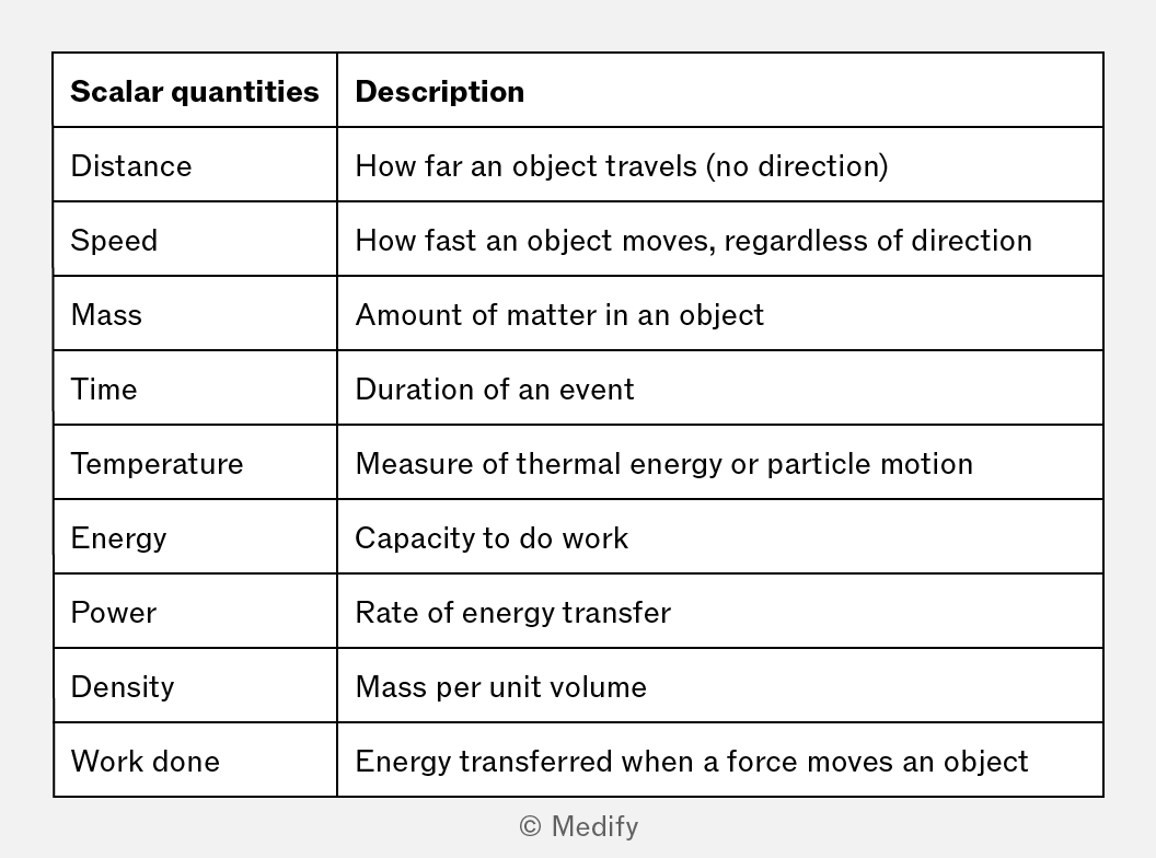
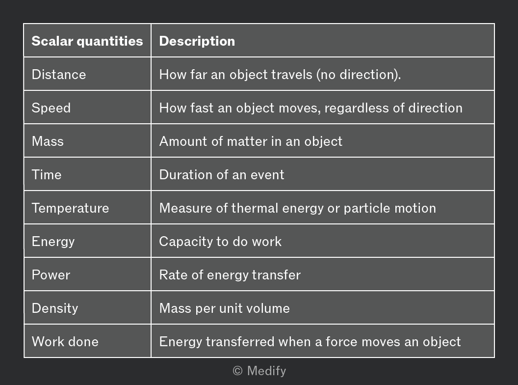
A table titled 'Scalar quantities' with two columns. The first column lists the quantities: Distance, Speed, Mass, Time, Temperature, Energy, Power, Density, Work done. The second column provides descriptions for each quantity: Distance - How far an object travels (no direction), Speed - How fast an object moves, regardless of direction, Mass - Amount of matter in an object, Time - Duration of an event, Temperature - Measure of thermal energy or particle motion, Energy - Capacity to do work, Power - Rate of energy transfer, Density - Mass per unit volume, Work done - Energy transferred when a force moves an object. The table is attributed to Medify.

An example of a scalar quantity is mass. The average mass of a human is which is just a value and has no direction.

Vector quantities have both magnitude and direction.

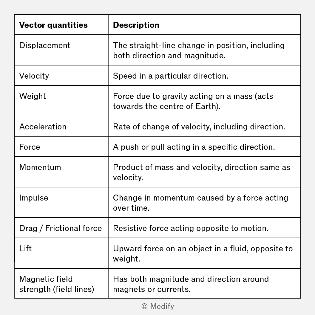
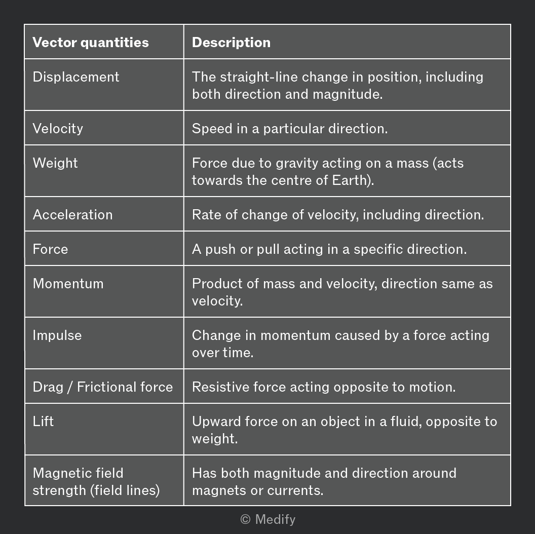
Vector quantities and their descriptions: Displacement - The straight-line change in position, including both direction and magnitude. Velocity - Speed in a particular direction. Weight - Force due to gravity acting on a mass (acts towards the centre of Earth). Acceleration - Rate of change of velocity, including direction. Force - A push or pull acting in a specific direction. Momentum - Product of mass and velocity, direction same as velocity. Impulse - Change in momentum caused by a force acting over time. Drag / Frictional force - Resistive force acting opposite to motion. Lift - Upward force on an object in a fluid, opposite to weight. Magnetic field strength (field lines) - Has both magnitude and direction around magnets or currents.

An example of a vector quantity is force. A person of mass standing on the surface of Earth feels a force due to their weight with magnitude (where is the gravitational field strength) and direction pointing towards the Earth’s centre.

Scalar quantities with the same units can be added or subtracted from each other.

For example, two rulers placed end to end have a total length:

Scalar quantities can be multiplied or divided by other scalar quantities. In these cases, the units of the scalar quantities may differ.

For example, speed is a scalar quantity given by the equation:

Distance has units and time has units giving the total units of speed as

Since a scalar quantity is just a number, a scalar quantity multiplied by another always gives a scalar quantity.

A scalar quantity multiplied by a vector quantity gives a vector quantity.

For example, Newton’s second law states that:

Where:

force is a vector quantity,
mass, is a scalar quantity, and
acceleration, is a vector quantity.

A vector can be represented visually by an arrow:

The length of the arrow is proportional to the vector magnitude.
The arrow points in the direction of the vector.
A vector is usually written with an arrow above the letter:
A vector can also be represented by an underlined letter:

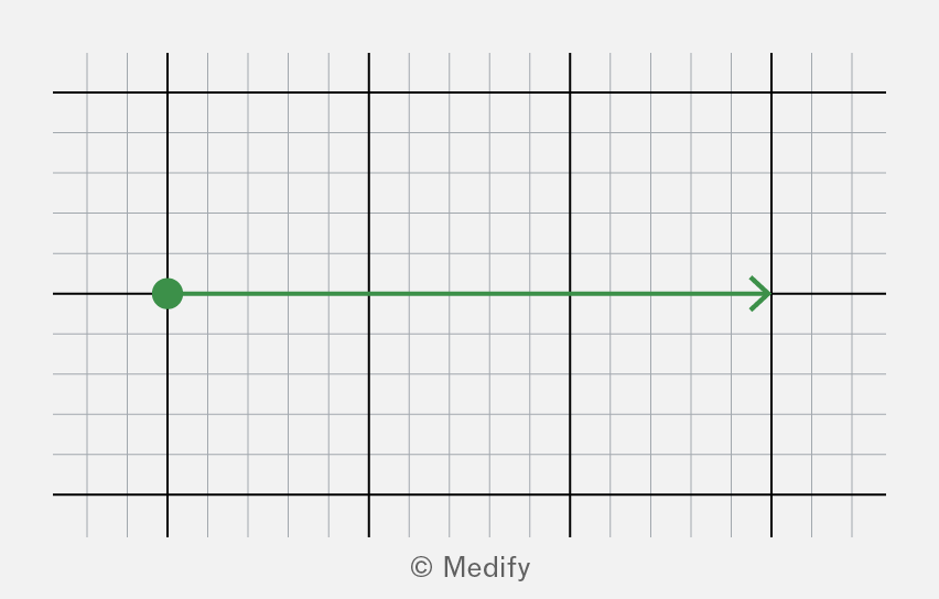
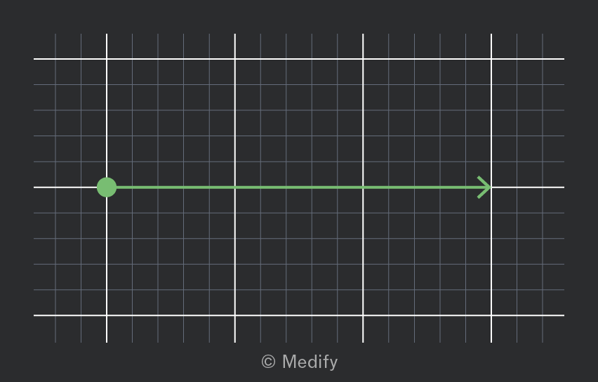
A grid with horizontal and vertical lines. A green line extends horizontally from a green dot on the left to an arrow pointing right.

The diagram above shows a force vector drawn on paper with squares:

If the scale is then the force has a magnitude
The direction of the arrow indicates that the force is directed to the right.

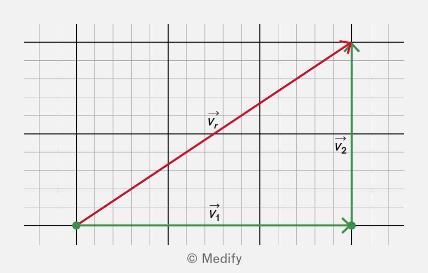
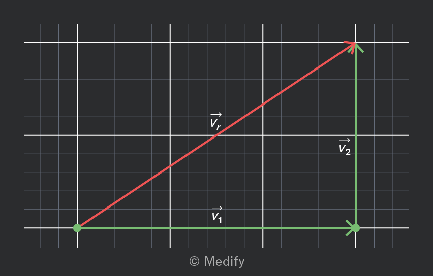
The diagram below shows the addition of two vectors and

Vectors can be added by placing the arrows end to end, as shown below.
The resultant vector can be found by drawing an arrow from the start of the first vector arrow to the end of the second arrow.

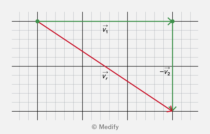
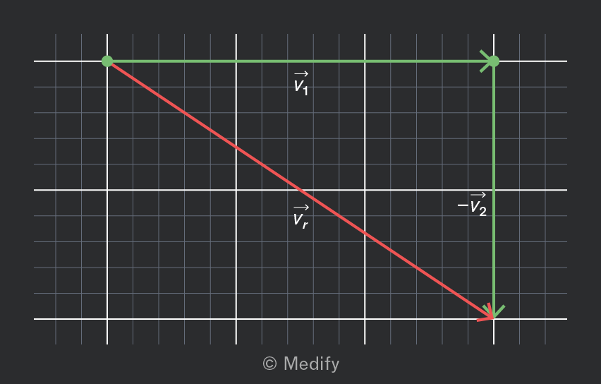
A graph with a grid background showing three vectors: a red vector labeled v→r, a green vector labeled v→1, and another green vector labeled v→2. The vectors originate from a green point at the bottom left corner of the graph.

The diagram below shows the subtraction of two vectors from

To subtract one vector from another, treat it as adding the negative: . This means reversing the direction of to get , then adding it to end-to-end.
The resultant vector runs from the tail of the first vector to the tip of the reversed vector . It represents the difference between the two original vectors, both in magnitude and direction

A graph with a grid background showing two vectors. The first vector, represented by an arrow labeled →v1, is green and moves horizontally to the right. The second vector, represented by an arrow labeled →vr, is red and moves diagonally downward to the left. There is also an arrow labeled −→v2, which is green and moves vertically downward.

The magnitude of the resultant vector, can be found from Pythagoras’ theorem:

Where and are the magnitudes of the two perpendicular vectors.

The diagram below shows the vector addition of two perpendicular displacement vectors.

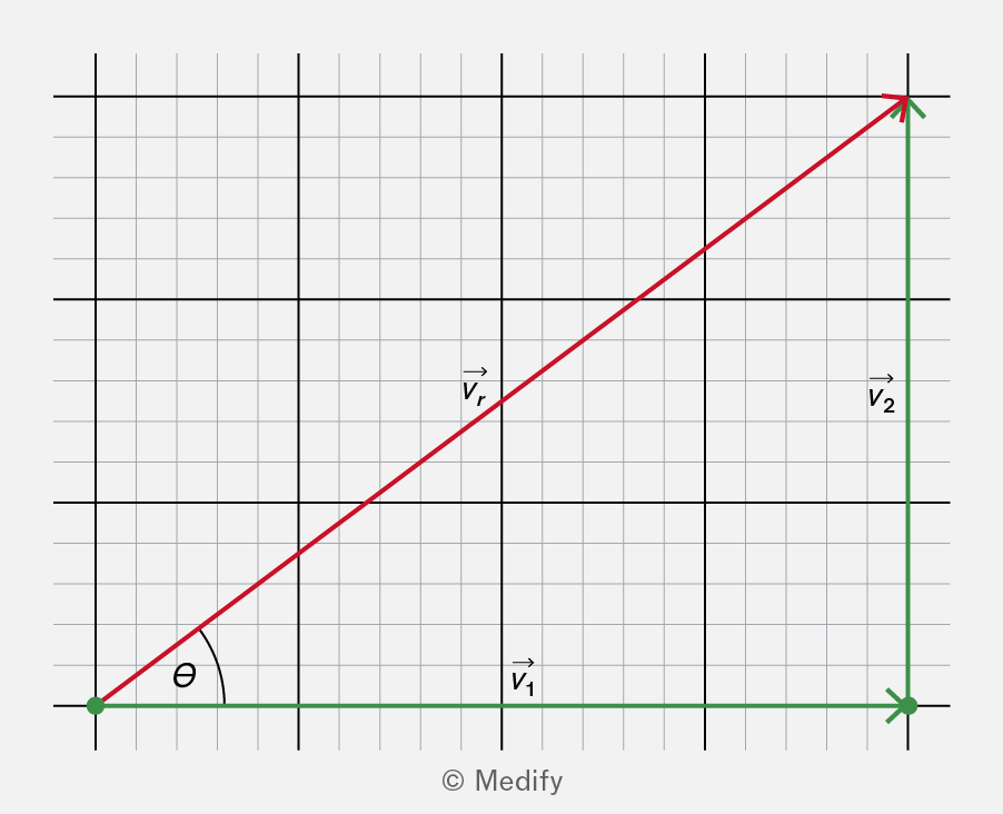
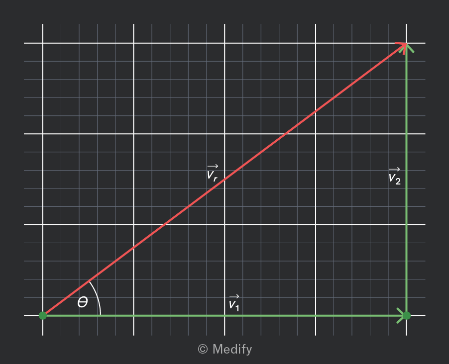
A graph showing vectors in a coordinate system. The red vector is labeled with v_r, and it points diagonally upwards. The green vector is labeled with v_1 and v_2, pointing horizontally and vertically, respectively. An angle θ is indicated at the origin.

In the diagram above, and so:

Trigonometric relationships can be used to determine the direction of a resultant vector that is formed by two vectors and acting perpendicularly to one another.

For the diagram below, the angle, of the resultant vector to the horizontal can be found from:

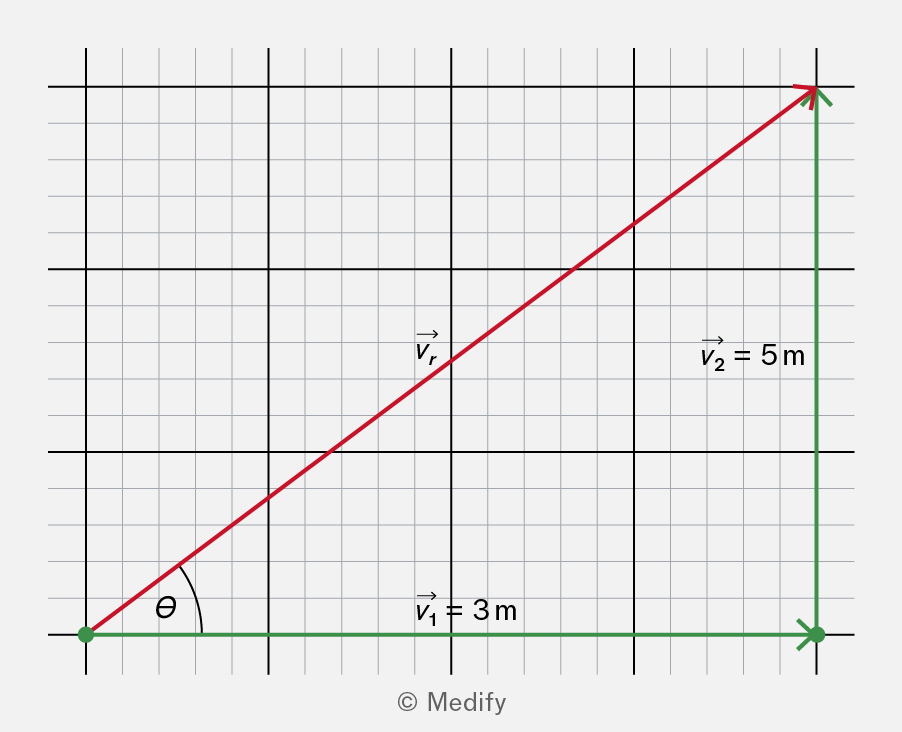
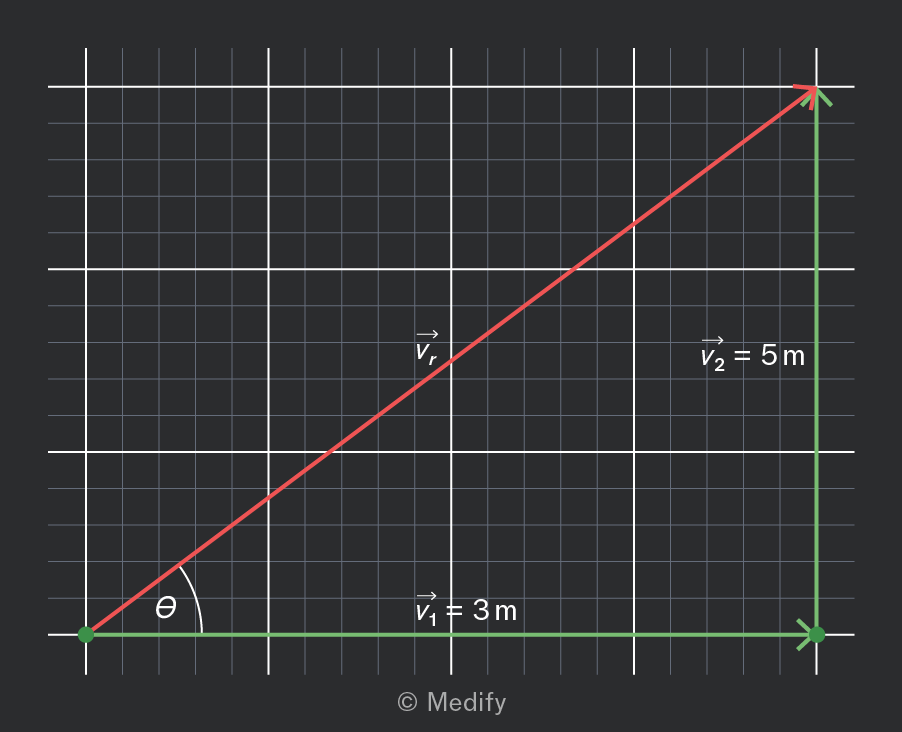
A graph showing two vectors. The red vector labeled v_r points diagonally, with v_2 = 5 m at the top right and v_1 = 3 m at the bottom left. An angle θ is indicated at the origin.

In the diagram above is opposite the angle while is adjacent. Therefore, the angle can be calculated as follows:

It is useful to note that the magnitude and direction of any resultant vector can also be calculated for any coplanar vector using the cosine rule and the sine rule.

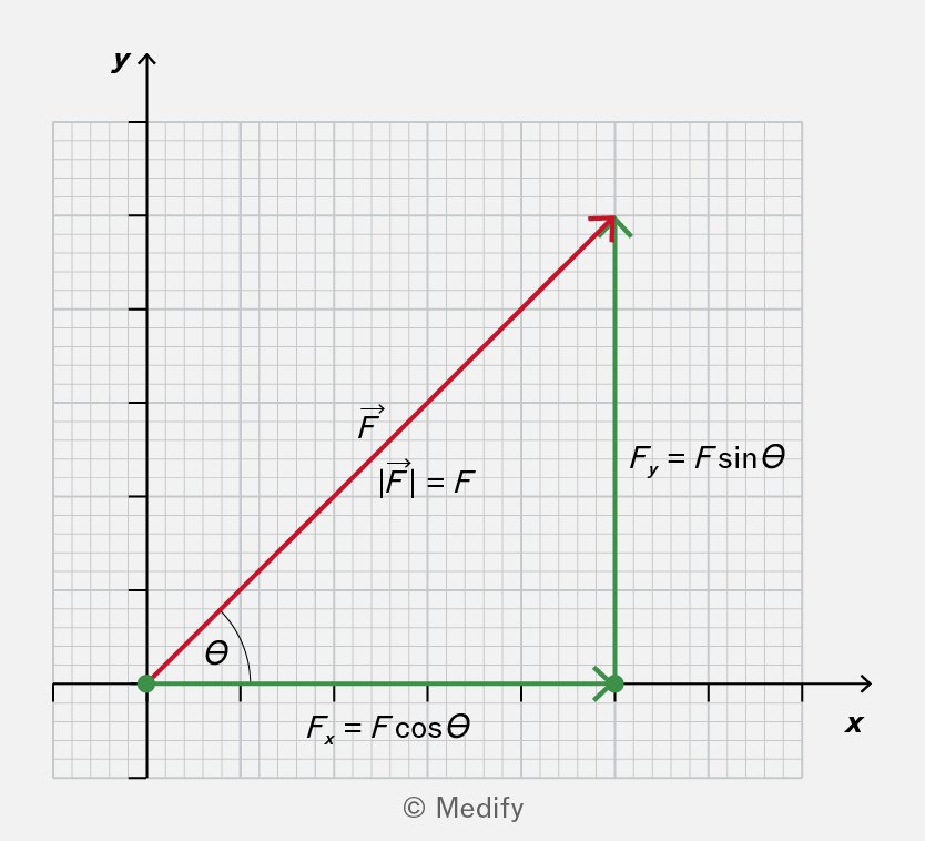
A vector can be resolved into its perpendicular components.

A force acting in the plane may be resolved into its and components. For a force with magnitude pointing at an angle to the X axis:

The horizontal component magnitude is
The vertical component magnitude is

A graph showing a vector in a Cartesian coordinate system. The vector is represented by a red arrow labeled F with its magnitude |F| = F. The angle θ is indicated at the base of the vector. The horizontal component of the vector is labeled Fx = F cos θ, and the vertical component is labeled Fy = F sin θ. The y-axis is vertical and the x-axis is horizontal.

There are many contexts where resolving a vector into its perpendicular components is useful, often when an object is constrained to move in one direction or when only one direction of the vector is relevant:

An example of this is in foot races, the wind velocity component parallel to the track must be calculated to determine the headwind or tailwind during a race.

Another example of this is projectile motion, in which an object is acted on by gravity so that its horizontal velocity component remains the same (ignoring air resistance) but its vertical velocity component varies.

Foundations in physics

On this page

Physical quantities

Question walkthrough

Estimating Gravity on Mars from Force and Mass

SI units

Measurements and uncertainties

Scalars and vectors