Analogue signal processing (3.13.3)

A filter is constructed using an LC circuit, i.e. an inductor-capacitance circuit (also known as an LC resonant circuit).

An LC circuit consists of an inductor L connected in parallel to a capacitor C as shown in the circuit diagram below. The setup allows for the filtering of frequencies when processing analogue signals.

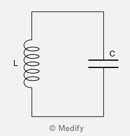
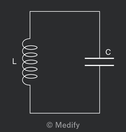
An inductor is a circuit component that stores energy in the form of a magnetic field. It consists of a coil of wire that is sometimes wrapped around an iron core.

The diagram below shows how an LC circuit works.

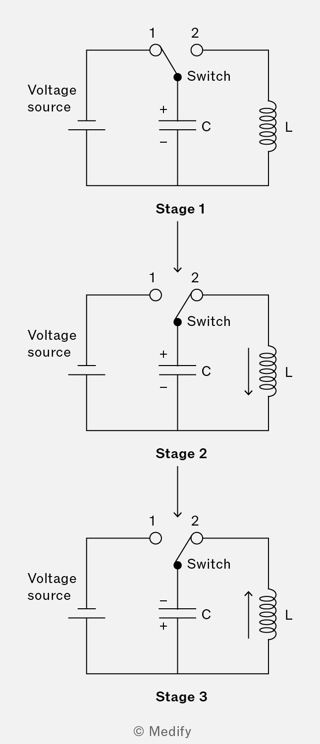
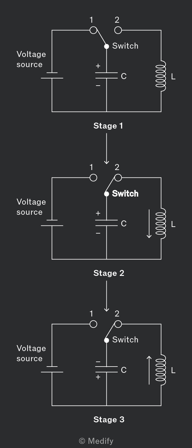
• Stage 1: The switch is in Position 1, and a potential difference will be applied across the capacitor plates by the voltage source. So, the capacitor charges and stores electrostatic potential energy due to the accumulation of charge at the plates.

• Stage 2: The switch is moved to Position 2. Current from the capacitor will now flow through the inductor and generate a magnetic field. As the capacitor loses charge, electrostatic potential energy is converted into magnetic field energy in the inductor.

• Stage 3: When the capacitor is fully discharged, no more current flows and the magnetic field generated in the inductor ceases. So, an emf is induced, creating a current in the opposite direction.
  • The capacitor charges with opposite polarity, converting magnetic energy back into electrostatic energy. When the capacitor is fully charged, the cycle repeats, and the capacitor discharges current through the inductor in the opposite direction.

The repeating cycle of charging and discharging (and the conversion of energy) in an LC circuit is described as an oscillating LC circuit.

There are four stages involved in an oscillating LC circuit:

1. Charging of the capacitor.
2. Discharging of the capacitor and generation of a magnetic field in the inductor.
3. Recharging of the capacitor with opposite polarity. Loss of magnetic field in the inductor.
4. Repeat: discharging of the capacitor and generation of a magnetic field in the inductor

An oscillating LC circuit is analogous to that of an oscillating mass on a spring.

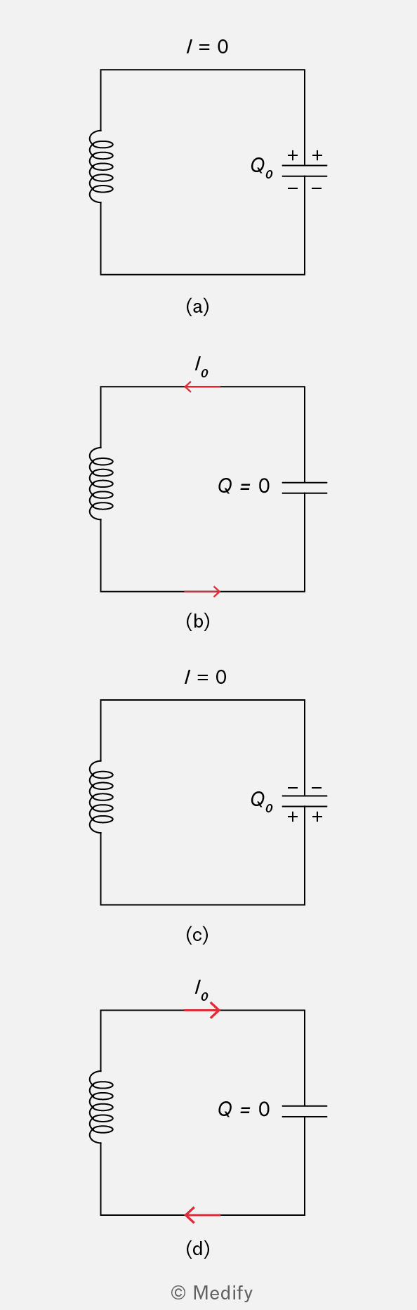
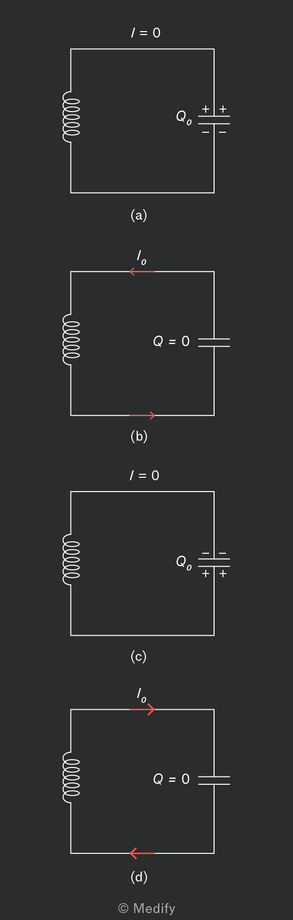
An oscillating LC circuit repeatedly charges and discharges its capacitor. The first of four stages involves charging the capacitor.

Before the switch is closed, a charge is stored in the capacitor. Therefore, there is only electrostatic potential energy stored in the electric field of the capacitor.

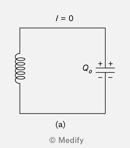
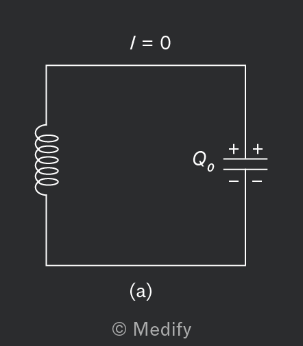
This is equivalent to a spring stretched to its maximum displacement – maximum elastic potential energy is stored in the spring.

An oscillating LC circuit repeatedly charges and discharges its capacitor. The second of four stages starts with closing the switch. The capacitor discharges and creates a current

This creates a magnetic field in the inductor – there is a transfer of electrostatic potential energy in the capacitor to magnetic field energy in the inductor. Eventually, all the energy in the circuit is stored as magnetic field energy.

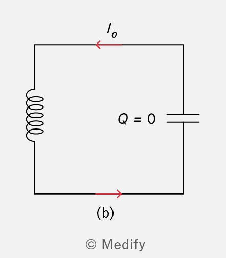
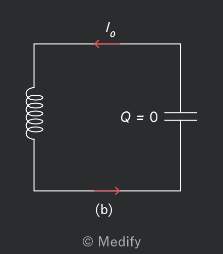
This is equivalent to the spring at its equilibrium level, i.e. when the mass is moving with maximum velocity – maximum kinetic energy is stored in the mass.

An oscillating LC circuit repeatedly charges and discharges. The third stage out of four recharges the capacitor, except with opposite polarity.

As the capacitor becomes fully discharged, the current continues to flow for a short time due to the inductor’s magnetic field resisting changes in current. This current begins to charge the capacitor with the opposite polarity. The magnetic field energy in the inductor is converted back into electrostatic potential energy in the capacitor.

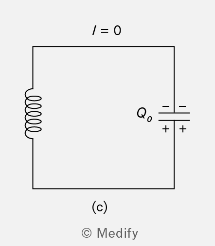
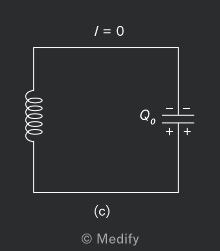
This is equivalent to the spring reaching maximum displacement on the other side of the equilibrium position – maximum elastic potential energy is stored again.

An oscillating LC circuit repeatedly charges and discharges its capacitor. The whole process repeats in the final stage. The capacitor discharges again, creating a current in the opposite direction, which generates a magnetic field in the inductor. Energy continuously oscillates between the electric field of the capacitor and the magnetic field of the inductor.

As a result, an oscillating current and charge are present in the circuit, as the capacitor continuously charges and discharges, as shown in the graph below.

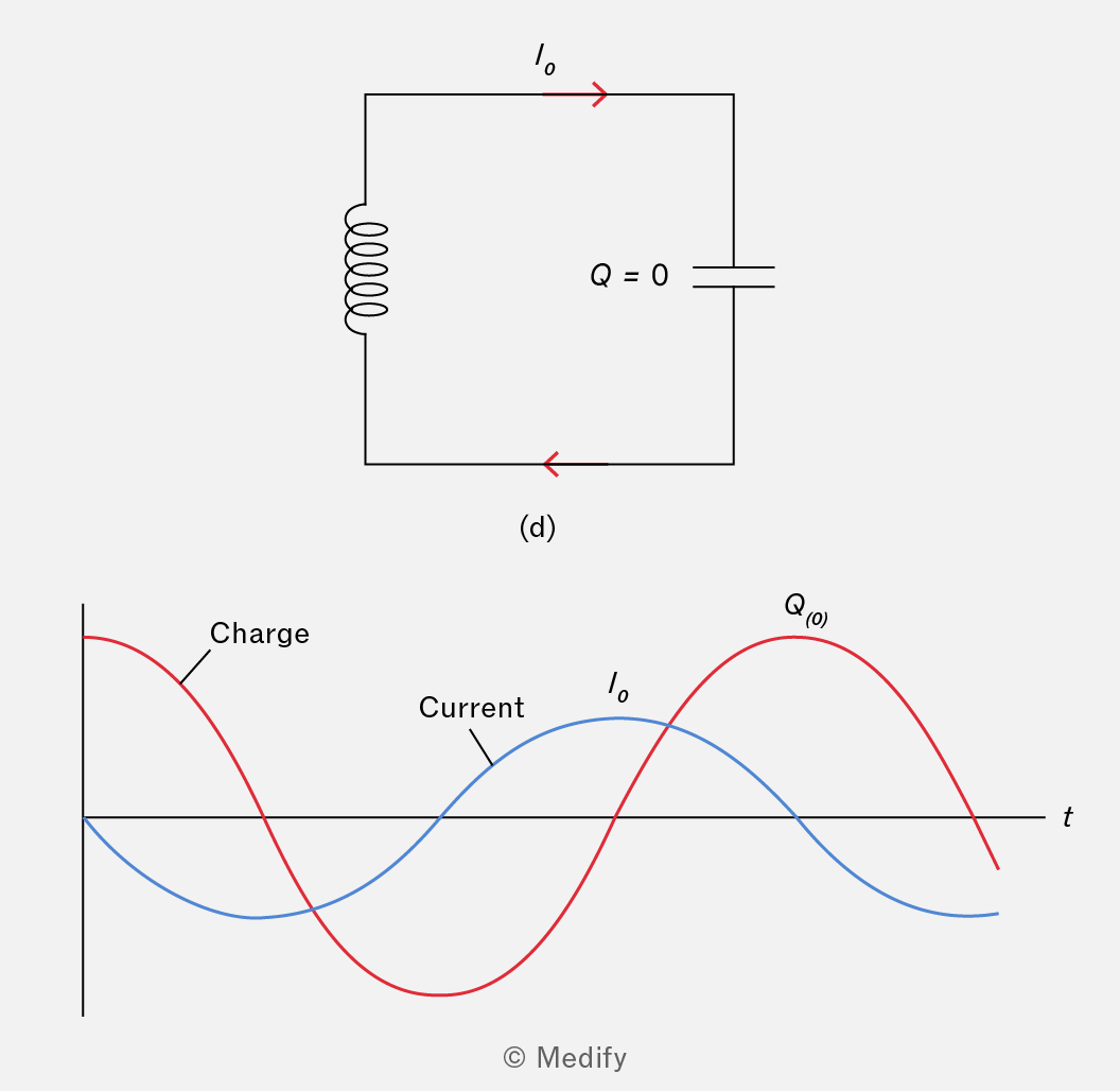
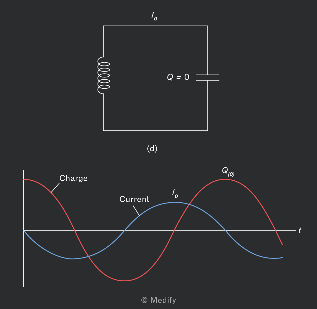
This behaviour is observed in the mass-spring system – energy oscillates between elastic potential energy and kinetic energy.

Oscillations in a parallel LC circuit can be driven by an alternating voltage source, as shown below.

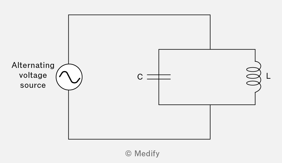
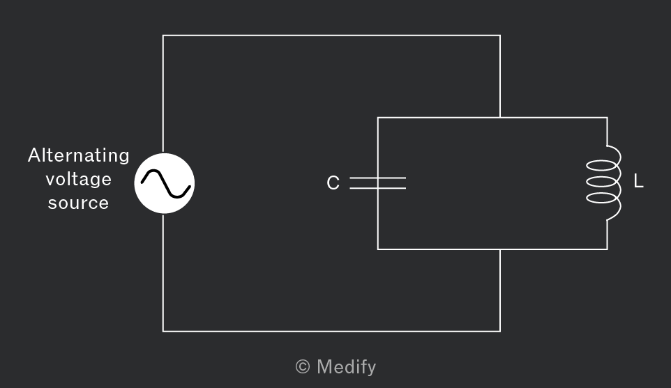
The charge oscillates back and forth between the capacitor and the inductor at the same frequency as the alternating source. If the voltage source frequency matches the LC circuit’s natural frequency, resonance will occur. As a result, the current will increase at that frequency.

The resonant frequency of a parallel LC circuit is calculated by:

Where:

• is the inductance (H), and
• is the capacitance (F).

In a parallel LC circuit, maximum energy is stored at the resonant frequency, and the voltage across the circuit reaches its peak value at resonance. The graph below shows the energy response curve of a parallel LC circuit:

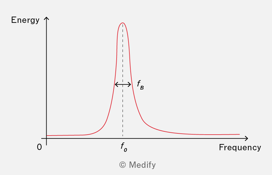
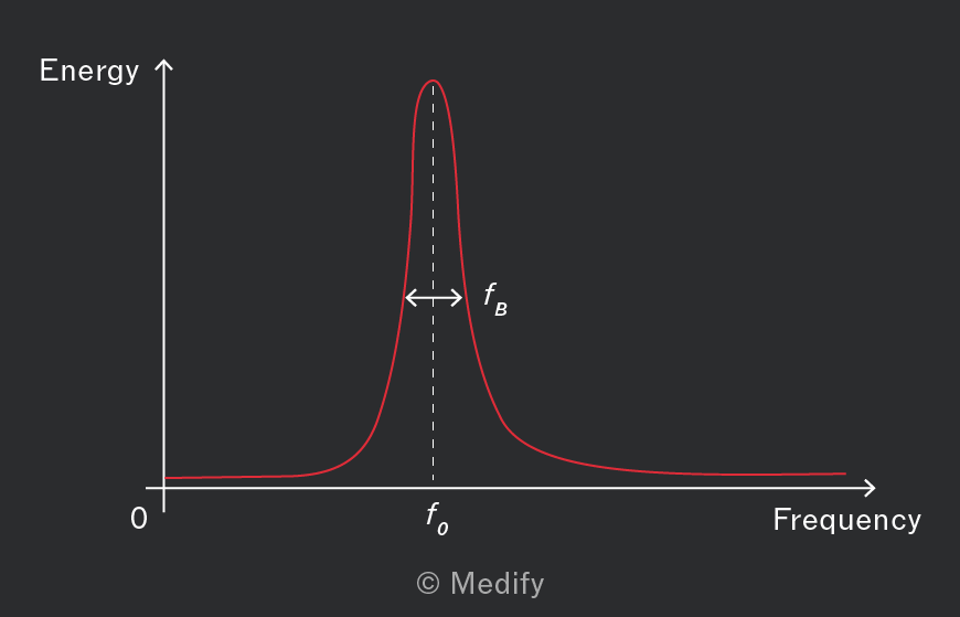
The resonant peak has a bandwidth and is a measure of how sharp the peak is. The bandwidth represents the frequency range at which 50% of the maximum energy is located.

The (quality) factor of a resonant LC circuit is defined as:

LC circuits with a high factor have narrow bandwidths, and LC circuits with a low factor have a wide bandwidth.

An LC resonant circuit can be used as a tuning filter to detect, for example, radio broadcasts.

An aerial detects the electric field component of radio waves at a particular frequency, creating an alternating voltage that produces a current through the connected circuit. The circuit includes a parallel LC resonator.

The circuit diagram below shows an LC resonator circuit in a radio aerial.

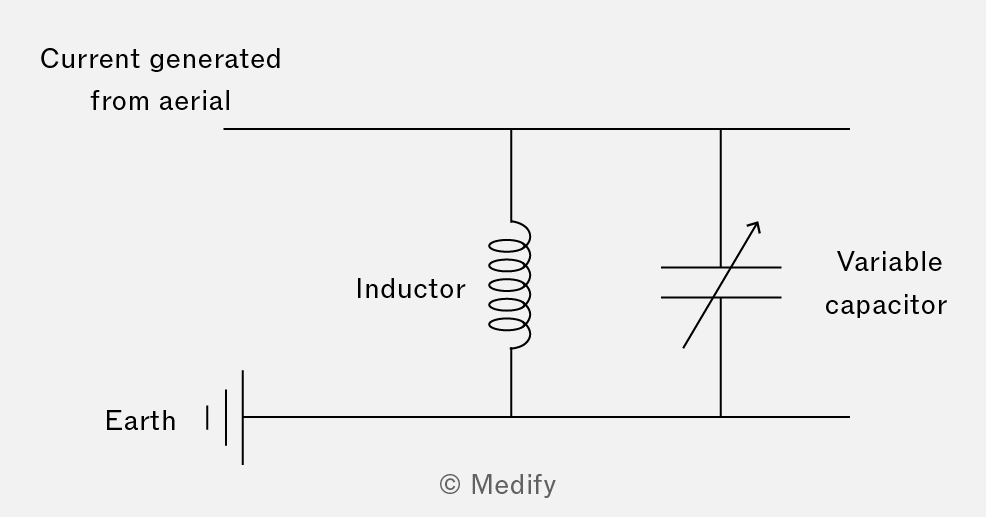
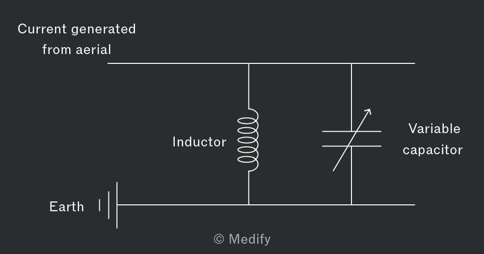
Instead of a fixed capacitor, a variable capacitor is used, allowing the LC circuit to be tuned. The circuit’s resonant frequency is adjusted to match that of the radio wave, thereby filtering out other transmitted frequencies. This creates a peak voltage response across the LC circuit. This voltage can be amplified and further processed to produce an output.

Amplifiers are devices that receive a weak signal and produce a stronger analogue signal.

The operational amplifier (op-amp) is an integrated circuit amplifier that can be configured in various ways to amplify analogue signals for different purposes.

The circuit symbol for the op-amp is shown below.

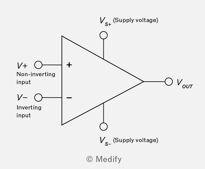
• At the non-inverting input , the output voltage changes in the same direction as the input signal applied to this terminal.

• At the inverting input , the output voltage changes in the opposite direction as the input signal applied to this terminal.

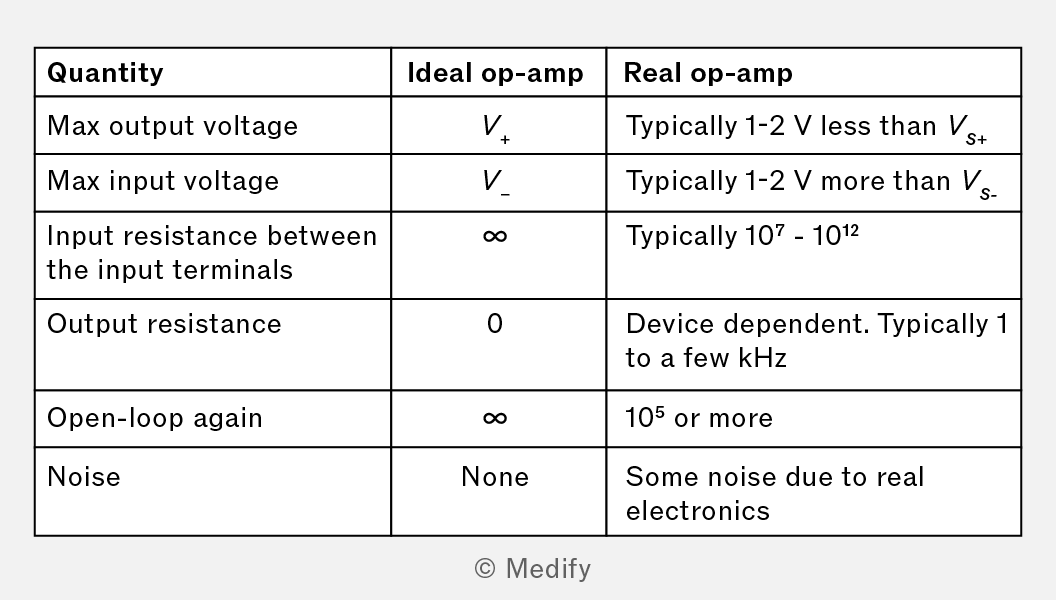
The characteristics of an ideal op-amp and a typical real op-amp are shown in the table below.

Op-amps have an open-loop output function, which is known as the transfer function:

Where:

• is the non-inverting input voltage, and
• is the inverting input voltage.

The op-amp amplifies the difference between the non-inverting and inverting inputs. The graph below shows the output voltage against the difference:

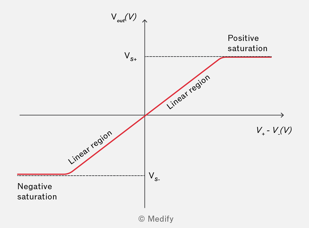
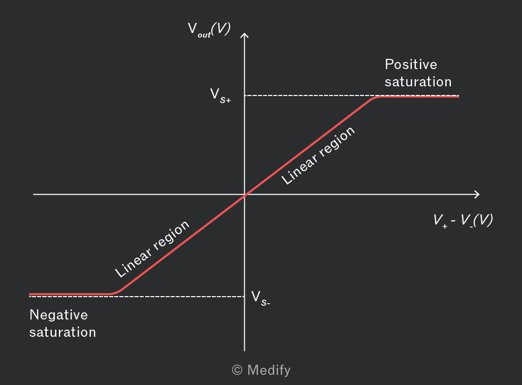
The output voltage is linear; however, it saturates at the supply voltages and This is due to the open-loop gain of the op-amp being high, which limits the value of the output voltage and results in a steep slope. The gradient of the slope is equal to

An op-amp amplifies the voltage difference between its inputs, making it suitable for voltage comparison, i.e. it can be used as a comparator.

The circuit diagram below shows the op-amp being used as a simple comparator.

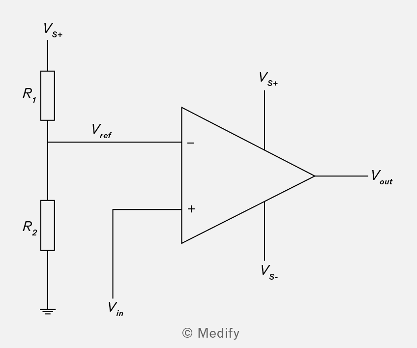
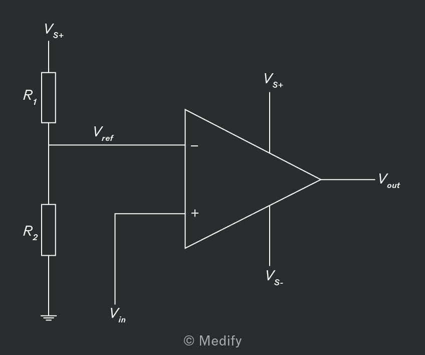
The two resistors form a potential divider with a reference voltage, connected to the inverting input. A varying voltage, is connected to the non-inverting input that is compared with

Since the open-loop gain of the amplifier is very large, the output voltage, will be saturated other than when the value of is equal to When the transfer function states that and, therefore, detects when is equal to